Static data
The foxes package comes with a set of data files whose main purpose is to serve for examples and tests. They are also a demonstration of the file formats that are required for input data. Such provided data files are often referred to as static data in foxes terminology.
Three different types of data are provided: Wind farm layout data, ambient states data, and power and thrust curve data.
import matplotlib.pyplot as plt

import foxes
import foxes.variables as FV
/home/runner/work/foxes/foxes/foxes/core/engine.py:4: TqdmExperimentalWarning: Using `tqdm.autonotebook.tqdm` in notebook mode. Use `tqdm.tqdm` instead to force console mode (e.g. in jupyter console)
  from tqdm.autonotebook import tqdm
Wind farm layout data
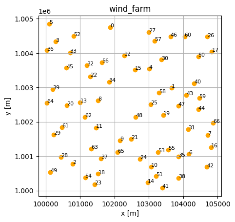
test_farm_67.csv
This is a wind farm with 67 turbines with randomly generated turbine coordinates. The file starts as follows:
index,label,x,y
0,T0,101872.70,1004753.57
1,T1,103659.97,1002993.29
2,T2,100780.09,1000779.97
3,T3,100290.42,1004330.88
4,T4,103005.58,1003540.36
5,T5,100102.92,1004849.55
6,T6,104162.21,1001061.70
...
The random layout looks like this:
farm = foxes.WindFarm()
foxes.input.farm_layout.add_from_file(
    farm, "test_farm_67.csv", turbine_models=[], verbosity=0
)
foxes.output.FarmLayoutOutput(farm).get_figure()
plt.show()
Ambient states data
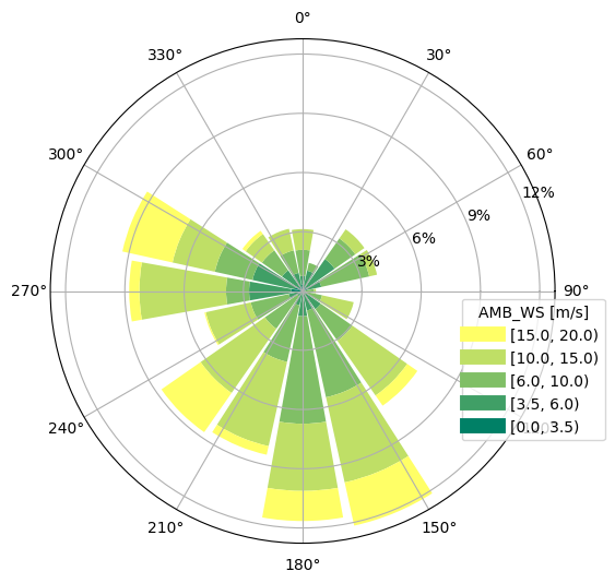
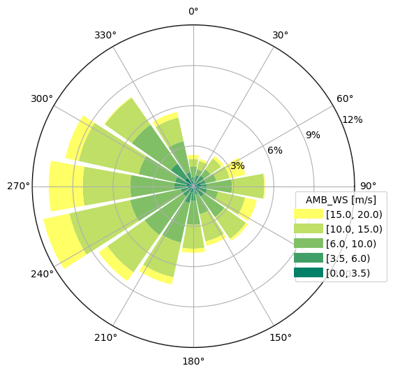
WRF-Timeseries-4464.csv.gz
This data represents a timeseries with 4464 entries as obtained by the mesoscale simulation software WRF at a single horizontal point with 8 different heights:
Time,WS-50,WS-75,...,WS-500,WD-50,WD-75,...,WD-500,TKE-50,TKE-75,...,TKE-500,RHO
2009-01-01 00:00:00,7.37214,7.42685,...,1.28838
...
2009-01-31 23:50:00,10.27767,10.36368,...,1.30095
At 100 m height the wind distribution looks like this:
states = foxes.input.states.MultiHeightTimeseries(
    data_source="WRF-Timeseries-4464.csv.gz",
    output_vars=[FV.WS, FV.WD, FV.TI, FV.RHO],
    heights=[50, 75, 90, 100, 150, 200, 250, 500],
    fixed_vars={FV.TI: 0.05},
)

o = foxes.output.StatesRosePlotOutput(states, point=[0.0, 0.0, 100.0])
o.get_figure(16, FV.AMB_WS, [0, 3.5, 6, 10, 15, 20], figsize=(6, 6))
plt.show()
DefaultEngine: Selecting engine 'single'
SingleChunkEngine: Calculating 4464 states for 1 turbines
SingleChunkEngine: Starting calculation using a single worker.
SingleChunkEngine: Completed all 1 chunks
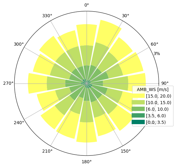
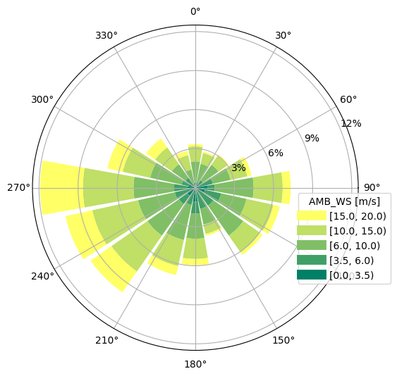
abl_states_6000.csv.gz
This file describes binnded atmospheric boundary layer data, including Monin-Obukhov length in the column mol:
state,ws,wd,ti,mol,weight
0,8.64,253.6,0.032,0.0,8.542331196166035e-05
1,10.65,207.8,0.145,0.0,0.0001230528308906
2,6.49,46.7,0.116,0.0,0.0001563449299843
3,15.72,314.4,0.048,0.0,6.618827331554488e-05
4,11.18,302.8,0.027,694.5,5.98695302482496e-05
...
The distribution is well populated for all wind directions:
states = foxes.input.states.StatesTable(
    data_source="abl_states_6000.csv.gz",
    output_vars=[FV.WS, FV.WD, FV.TI, FV.RHO, FV.MOL],
    var2col={FV.WS: "ws", FV.WD: "wd", FV.TI: "ti", FV.MOL: "mol"},
    fixed_vars={FV.RHO: 1.225, FV.Z0: 0.05, FV.H: 100.0},
    profiles={FV.WS: "ABLLogWsProfile"},
)

o = foxes.output.StatesRosePlotOutput(states, point=[0.0, 0.0, 100.0])
o.get_figure(16, FV.AMB_WS, [0, 3.5, 6, 10, 15, 20], figsize=(6, 6))
plt.show()
DefaultEngine: Selecting engine 'single'
SingleChunkEngine: Calculating 6000 states for 1 turbines
SingleChunkEngine: Starting calculation using a single worker.
SingleChunkEngine: Completed all 1 chunks
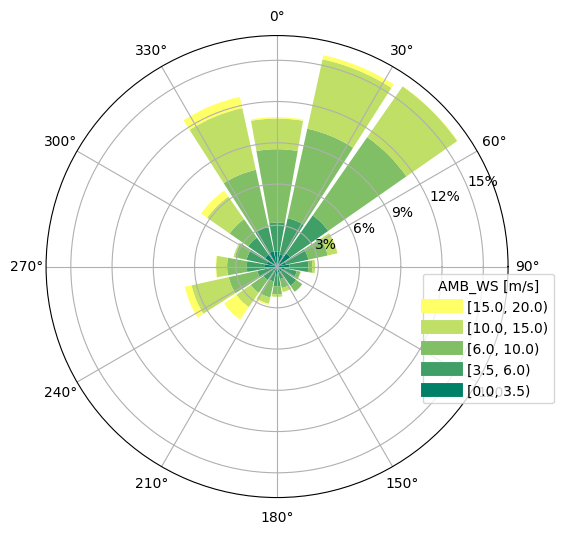
timeseries_3000.csv.gz
This is a timeseries with 3000 entries:
Time,WS,WD,TI,RHO
2018-09-30 15:00:00,24.29,172.9,0.05,1.27
2018-09-30 16:00:00,22.51,184.13,0.05,1.21
2018-09-30 17:00:00,10.52,198.5,0.04,1.24
2018-09-30 18:00:00,34.36,209.93,0.04,1.27
2018-09-30 19:00:00,31.78,217.35,0.04,1.23
2018-09-30 20:00:00,29.15,223.8,0.04,1.26
2018-09-30 21:00:00,25.68,227.6,0.02,1.24
...
The distribution is as follows:
states = foxes.input.states.Timeseries(
    data_source="timeseries_3000.csv.gz",
    output_vars=[FV.WS, FV.WD, FV.TI, FV.RHO],
)

o = foxes.output.StatesRosePlotOutput(states, point=[0.0, 0.0, 100.0])
o.get_figure(16, FV.AMB_WS, [0, 3.5, 6, 10, 15, 20], figsize=(6, 6))
plt.show()
DefaultEngine: Selecting engine 'single'
SingleChunkEngine: Calculating 3000 states for 1 turbines
SingleChunkEngine: Starting calculation using a single worker.
SingleChunkEngine: Completed all 1 chunks
timeseries_8000.csv.gz
This is a timeseries with 8000 entries:
Time,ws,wd,ti
2017-01-01 00:00:00,15.62,244.06,0.0504
2017-01-01 00:30:00,15.99,243.03,0.0514
2017-01-01 01:00:00,16.31,243.01,0.0522
2017-01-01 01:30:00,16.33,241.26,0.0523
2017-01-01 02:00:00,16.16,241.62,0.0518
2017-01-01 02:30:00,15.95,242.21,0.0513
...
The distribution is as follows:
states = foxes.input.states.Timeseries(
    data_source="timeseries_8000.csv.gz",
    output_vars=[FV.WS, FV.WD, FV.TI, FV.RHO],
    var2col={FV.WS: "ws", FV.WD: "wd", FV.TI: "ti"},
    fixed_vars={FV.RHO: 1.225},
)

o = foxes.output.StatesRosePlotOutput(states, point=[0.0, 0.0, 100.0])
o.get_figure(16, FV.AMB_WS, [0, 3.5, 6, 10, 15, 20], figsize=(6, 6))
plt.show()
DefaultEngine: Selecting engine 'single'
SingleChunkEngine: Calculating 8000 states for 1 turbines
SingleChunkEngine: Starting calculation using a single worker.
SingleChunkEngine: Completed all 1 chunks
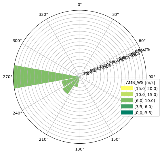
timeseries_100.csv.gz
A short timeseries with 100 entries and one minute time step, varying only wind direction:
Time,wd,ws
2023-07-07 12:00:00,270.0,6.0
2023-07-07 12:01:00,270.0,6.0
...
2023-07-07 12:20:00,270.0,6.0
2023-07-07 12:21:00,269.836,6.0
2023-07-07 12:22:00,269.344,6.0
2023-07-07 12:23:00,268.532,6.0
2023-07-07 12:24:00,267.406,6.0
2023-07-07 12:25:00,265.981,6.0
...
2023-07-07 13:39:00,270.0,6.0
The distribution is as follows:
states = foxes.input.states.Timeseries(
    data_source="timeseries_100.csv.gz",
    output_vars=[FV.WS, FV.WD, FV.TI, FV.RHO],
    var2col={FV.WS: "ws", FV.WD: "wd"},
    fixed_vars={FV.RHO: 1.225, FV.TI: 0.05},
)

o = foxes.output.StatesRosePlotOutput(states, point=[0.0, 0.0, 100.0])
o.get_figure(16, FV.AMB_WS, [0, 3.5, 6, 10, 15, 20], figsize=(6, 6))
plt.show()
DefaultEngine: Selecting engine 'single'
SingleChunkEngine: Calculating 100 states for 1 turbines
SingleChunkEngine: Starting calculation using a single worker.
SingleChunkEngine: Completed all 1 chunks
wind_rose_bremen.csv
This data file represents a (coarse) wind rose with 216 states, representing a site near Bremen, Germany. Each of the states consists of the wind direction and wind speed bin centres, and the respective statistical weight of the bin (normalized such that 1 represents 100%):
state,wd,ws,weight
0,0.0,3.5,0.00158
1,0.0,6.0,0.00244
2,0.0,8.5,0.00319
3,0.0,12.5,0.00367
4,0.0,17.5,0.00042
...
The distribution looks as follows:
states = foxes.input.states.StatesTable(
    data_source="wind_rose_bremen.csv",
    output_vars=[FV.WS, FV.WD, FV.TI, FV.RHO],
    var2col={FV.WS: "ws", FV.WD: "wd", FV.WEIGHT: "weight"},
    fixed_vars={FV.RHO: 1.225, FV.TI: 0.05},
)

o = foxes.output.StatesRosePlotOutput(states, point=[0.0, 0.0, 100.0])
o.get_figure(16, FV.AMB_WS, [0, 3.5, 6, 10, 15, 20], figsize=(6, 6))
plt.show()
DefaultEngine: Selecting engine 'single'
SingleChunkEngine: Calculating 216 states for 1 turbines
SingleChunkEngine: Starting calculation using a single worker.
SingleChunkEngine: Completed all 1 chunks
wind_rotation.nc
This is a very small example for inhomogeneous wind data, with 2 states, 4 points and 2 heights:
dimensions:
        state = 2 ;
        h = 2 ;
        y = 2 ;
        x = 2 ;
variables:
        int state(state) ;
        float h(h) ;
                h:units = "m" ;
                h:long_name = "Height" ;
        float y(y) ;
                y:units = "m" ;
        float x(x) ;
                x:units = "m" ;
        float ws(state, h, y, x) ;
                ws:units = "m/s" ;
                ws:long_name = "Wind speed" ;
        float wd(state, h, y, x) ;
                wd:units = "deg" ;
                wd:long_name = "Wind direction" ;

// global attributes:
                :title = "Wind Rotation example" ;
                :subtitle = "A single wind state with uniform wind speed and spatial wind direction changes" ;
                :author = "IWES" ;
                :date = "22.06.2021" ;
data:

 state = 0, 1 ;

 h = 0, 300 ;

 y = 0, 2500 ;

 x = 0, 2500 ;

 ws =
  9, 9,
  9, 9,
  9, 9,
  9, 9,
  9, 9,
  9, 9,
  9, 9,
  9, 9 ;

 wd =
  180, 270,
  220, 250,
  180, 270,
  220, 250,
  0, 120,
  30, 90,
  0, 120,
  30, 90 ;
Power and thrust curves
DTU-10MW-D178d3-H119.csv
This file represents the DTU 10 MW reference turbine:
mbook = foxes.models.ModelBook()
mbook.turbine_types["DTU10"] = foxes.models.turbine_types.PCtFile(
    "DTU-10MW-D178d3-H119.csv"
)

o = foxes.output.TurbineTypeCurves(mbook)
d = o.calc_plot_data("DTU10", [FV.P, FV.CT])
fig, axs = plt.subplots(1, 2, figsize=(10, 4))
o.plot_curves(d, axs=axs)
plt.show()
DefaultEngine: Selecting engine 'single'
SingleChunkEngine: Calculating 301 states for 1 turbines
SingleChunkEngine: Starting calculation using a single worker.
SingleChunkEngine: Completed all 1 chunks
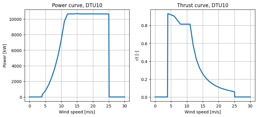
This turbine model is available in the default model book under the name DTU10MW.
IEA-15MW-D240-H150.csv
This file represents the IEA 15 MW reference turbine:
mbook = foxes.models.ModelBook()
mbook.turbine_types["IEA15"] = foxes.models.turbine_types.PCtFile(
    "IEA-15MW-D240-H150.csv"
)

o = foxes.output.TurbineTypeCurves(mbook)
d = o.calc_plot_data("IEA15", [FV.P, FV.CT])
fig, axs = plt.subplots(1, 2, figsize=(10, 4))
o.plot_curves(d, axs=axs)
plt.show()
DefaultEngine: Selecting engine 'single'
SingleChunkEngine: Calculating 301 states for 1 turbines
SingleChunkEngine: Starting calculation using a single worker.
SingleChunkEngine: Completed all 1 chunks
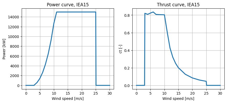
This turbine model is available in the default model book under the name IEA15MW.
IWT-7d5MW-D164-H100.csv
This file represents the IWES 7.5 MW reference turbine:
mbook = foxes.models.ModelBook()
mbook.turbine_types["IWT7.5"] = foxes.models.turbine_types.PCtFile(
    "IWT-7d5MW-D164-H100.csv"
)

o = foxes.output.TurbineTypeCurves(mbook)
d = o.calc_plot_data("IWT7.5", [FV.P, FV.CT])
fig, axs = plt.subplots(1, 2, figsize=(10, 4))
o.plot_curves(d, axs=axs)
plt.show()
DefaultEngine: Selecting engine 'single'
SingleChunkEngine: Calculating 301 states for 1 turbines
SingleChunkEngine: Starting calculation using a single worker.
SingleChunkEngine: Completed all 1 chunks
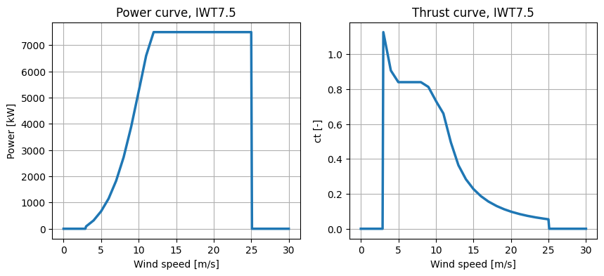
This turbine model is available in the default model book under the name IWT7.5MW.
NREL-5MW-D126-H90.csv
This file represents the NREL 5 MW reference turbine:
mbook = foxes.models.ModelBook()
mbook.turbine_types["NREL5"] = foxes.models.turbine_types.PCtFile(
    "NREL-5MW-D126-H90.csv"
)

o = foxes.output.TurbineTypeCurves(mbook)
d = o.calc_plot_data("NREL5", [FV.P, FV.CT])
fig, axs = plt.subplots(1, 2, figsize=(10, 4))
o.plot_curves(d, axs=axs)
plt.show()
DefaultEngine: Selecting engine 'single'
SingleChunkEngine: Calculating 301 states for 1 turbines
SingleChunkEngine: Starting calculation using a single worker.
SingleChunkEngine: Completed all 1 chunks
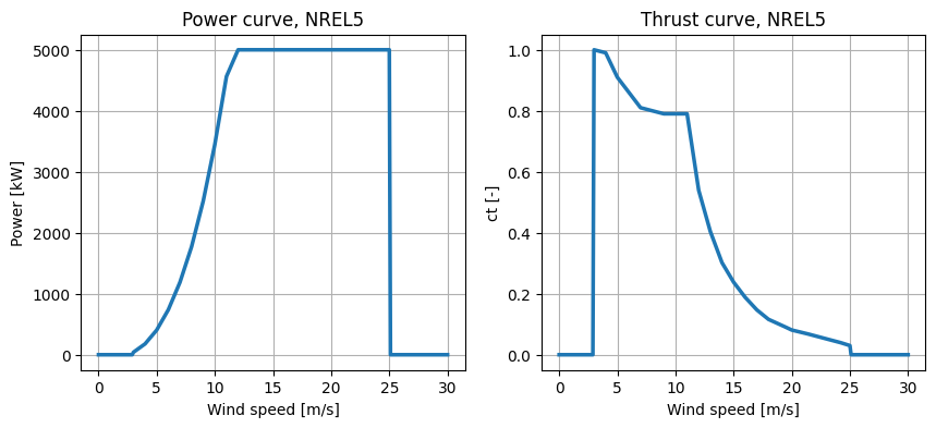
This turbine model is available in the default model book under the name NREL5MW.
File paths
The available static data files can be listed by creating a StaticData object:
import foxes
dbook = foxes.StaticData()

print("Farm:\n", dbook.toc(foxes.FARM))
print("\nStates:\n", dbook.toc(foxes.STATES))
print("\nCurves:\n", dbook.toc(foxes.PCTCURVE))
Farm:
 ['test_farm_67.csv']

States:
 ['10s_TEST.csv', 'WRF-Timeseries-3000.nc', 'WRF-Timeseries-4464.csv.gz', 'abl_states_6000.csv.gz', 'point_cloud_100.nc', 'target_grid_icon_eu_R03B08_nordsee.txt', 'target_grid_icon_eu_R03B08_ostsee.txt', 'timeseries_100.csv.gz', 'timeseries_3000.csv.gz', 'timeseries_8000.csv.gz', 'weibull_cloud_4.nc', 'weibull_grid.nc', 'weibull_sectors_12.csv', 'weibull_sectors_12.nc', 'wind_rose_bremen.csv', 'wind_rotation.nc', 'winds100.tab']

Curves:
 ['DTU-10MW-D178d3-H119.csv', 'IEA-15MW-D240-H150.csv', 'IWT-7d5MW-D164-H100.csv', 'NREL-5MW-D126-H90.csv']
Note that the toc function requires as argument one of the three data categories. For each of the mentioned files we can then get the path in the local system:
path = dbook.get_file_path(foxes.FARM, "test_farm_67.csv")
print(type(path), ":", path.relative_to(path.parents[3]))
<class 'pathlib.PosixPath'> : foxes/data/farms/test_farm_67.csv
The path is a full PosixPath object here, but only parts of it are shown in the printout (feel invited to print the complete file location when running this example yourself, simply by print(path)).