Parallelization
Even for large cases foxes calculations are fast, thanks to
Vectorization: The states (and also the points, in the case of data calculation at evaluation points) are split into so-called chunks, which are sub-arrays of the large original data.
Parallelization: These chunks are being sent to individual processes for calculation. Those calculations can be carried out simultaneously, i.e., in parallel.
Vectorization and parallelization are managed by so-called engines in foxes. If you do not explicitly specify the engine, a default will be chosen. This means that even if you do not know or care about foxes engines, your calculations will be vectorized and parallelized.
Available engines
These are the currently available engines, where each can be addressed by the short name or the full class name:
Short name |
Class name |
Base package |
Description |
|---|---|---|---|
threads |
ThreadsEngine |
Runs on a workstation/laptop, sends chunks to threads |
|
process |
ProcessEngine |
Runs on a workstation/laptop, sends chunks to parallel processes |
|
multiprocess |
MultiprocessEngine |
Runs on a workstation/laptop, sends chunks to parallel processes |
|
ray |
RayEngine |
Runs on a workstation/laptop, sends chunks to parallel processes |
|
dask |
DaskEngine |
Runs on a workstation/laptop, using processes or threads |
|
local_cluster |
LocalClusterEngine |
Runs on a workstation/laptop, creates a virtual local cluster |
|
slurm_cluster |
SlurmClusterEngine |
Runs on a multi-node HPC cluster which is using SLURM |
|
mpi |
MPIEngine |
Runs on laptop/workstation/cluster, also supports multi-node runs |
|
numpy |
NumpyEngine |
Runs a loop over chunks, without parallelization |
|
single |
SingleChunkEngine |
Runs all in a single chunk, without parallelization |
|
default |
DefaultEngine |
Runs either the |
Note that the external packages are not installed by default. You can install them manually on demand, or use the option pip install foxes[eng] for the complete installation of all requirements of the complete list of engines.
Furthermore, scripts that use the mpi engine have to be started in a special way. For example, when running a script named run.py on 12 processors, the terminal command is
mpiexec -n 12 python -m mpi4py.futures run.py
Default engine
Let’s start by importing foxes and other required packages:
import matplotlib.pyplot as plt

import foxes
import foxes.variables as FV
/home/runner/work/foxes/foxes/foxes/core/engine.py:4: TqdmExperimentalWarning: Using `tqdm.autonotebook.tqdm` in notebook mode. Use `tqdm.tqdm` instead to force console mode (e.g. in jupyter console)
  from tqdm.autonotebook import tqdm
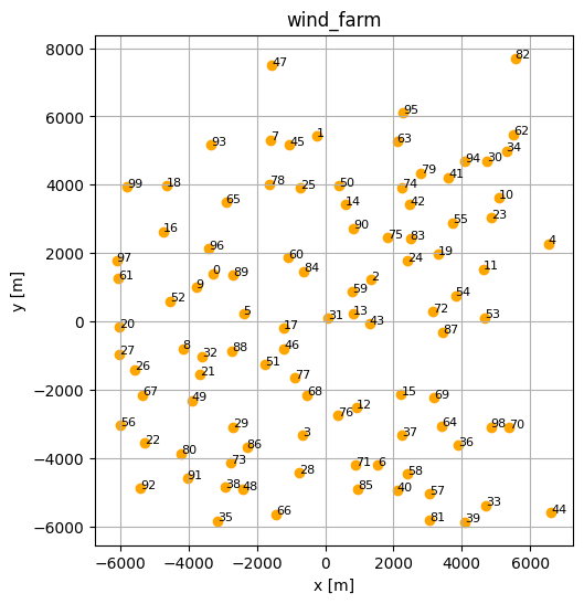
Next, we create a random wind farm and a random time series:
n_times = 5000
n_turbines = 100
seed = 42

sdata = foxes.input.states.create.random_timseries_data(
    n_times,
    seed=seed,
)
states = foxes.input.states.Timeseries(
    data_source=sdata,
    output_vars=[FV.WS, FV.WD, FV.TI, FV.RHO],
    fixed_vars={FV.RHO: 1.225, FV.TI: 0.02},
)

farm = foxes.WindFarm()
foxes.input.farm_layout.add_random(
    farm, n_turbines, min_dist=500, turbine_models=["DTU10MW"], seed=seed, verbosity=0
)
sdata
| WS | WD | |
|---|---|---|
| Time | ||
| 2000-01-01 00:00:00 | 11.236204 | 141.708787 |
| 2000-01-01 01:00:00 | 28.521429 | 170.436837 |
| 2000-01-01 02:00:00 | 21.959818 | 307.637062 |
| 2000-01-01 03:00:00 | 17.959755 | 122.401579 |
| 2000-01-01 04:00:00 | 4.680559 | 313.073887 |
| ... | ... | ... |
| 2000-07-27 03:00:00 | 26.921920 | 308.756156 |
| 2000-07-27 04:00:00 | 3.581430 | 323.103181 |
| 2000-07-27 05:00:00 | 9.835285 | 340.814849 |
| 2000-07-27 06:00:00 | 24.472361 | 143.095677 |
| 2000-07-27 07:00:00 | 17.919371 | 78.170545 |
5000 rows × 2 columns
foxes.output.FarmLayoutOutput(farm).get_figure(figsize=(6, 6))
plt.show()
You can run the wind farm calculations by simply creating an algorithm and calling farm_calc:
algo = foxes.algorithms.Downwind(
    farm,
    states,
    wake_models=["Bastankhah2014_linear_k004"],
    verbosity=1,
)
farm_results = algo.calc_farm()
farm_results.to_dataframe()
Initializing model 'Timeseries'

Initializing algorithm 'Downwind'

------------------------------------------------------------
  Algorithm: Downwind
  Running Downwind: calc_farm
------------------------------------------------------------
  n_states : 5000
  n_turbines: 100
------------------------------------------------------------
  states    : Timeseries()
  rotor     : CentreRotor()
  controller: BasicFarmController()
  deflection: NoDeflection()
  wake frame: RotorWD()
  wake lngth: None
------------------------------------------------------------
  wakes:
    0) Bastankhah2014_linear_k004: Bastankhah2014(ws_linear, induction=Madsen, k=0.04)
------------------------------------------------------------
  partial wakes:
    0) Bastankhah2014_linear_k004: axiwake6, PartialAxiwake(n=6)
------------------------------------------------------------
  turbine models:
    0) DTU10MW: PCtFile(D=178.3, H=119.0, P_nominal=10000.0, P_unit=kW, rho=1.225, var_ws_ct=REWS2, var_ws_P=REWS3)
------------------------------------------------------------


--------------------------------------------------
  Model oder
--------------------------------------------------
00) basic_ctrl
01) InitFarmData
02) centre
03) basic_ctrl
  03.0) Post-rotor: DTU10MW
04) SetAmbFarmResults
05) FarmWakesCalculation
06) ReorderFarmOutput
--------------------------------------------------


Input data:

 <xarray.Dataset> Size: 620kB
Dimensions:          (state: 5000, Timeseries_vars: 2, turbine: 100, tmodels: 1)
Coordinates:
  * state            (state) datetime64[ns] 40kB 2000-01-01 ... 2000-07-27T07...
  * Timeseries_vars  (Timeseries_vars) <U2 16B 'WD' 'WS'
  * tmodels          (tmodels) <U7 28B 'DTU10MW'
Dimensions without coordinates: turbine
Data variables:
    Timeseries_data  (state, Timeseries_vars) float64 80kB 141.7 11.24 ... 17.92
    tmodel_sels      (state, turbine, tmodels) bool 500kB True True ... True


Farm variables: AMB_CT, AMB_P, AMB_REWS, AMB_REWS2, AMB_REWS3, AMB_RHO, AMB_TI, AMB_WD, AMB_YAW, CT, D, H, P, REWS, REWS2, REWS3, RHO, TI, WD, X, Y, YAW, order, order_inv, order_ssel, weight

Output variables: AMB_CT, AMB_P, AMB_REWS, AMB_REWS2, AMB_REWS3, AMB_RHO, AMB_TI, AMB_WD, AMB_YAW, CT, D, H, P, REWS, REWS2, REWS3, RHO, TI, WD, X, Y, YAW, order, order_inv, order_ssel, weight
DefaultEngine: Selecting engine 'process'
ProcessEngine: Calculating 5000 states for 100 turbines
ProcessEngine: Starting calculation using 3 workers, for 3 states chunks.
ProcessEngine: Completed all 3 chunks
| AMB_CT | AMB_P | AMB_REWS | AMB_REWS2 | AMB_REWS3 | AMB_RHO | AMB_TI | AMB_WD | AMB_YAW | CT | ... | TI | WD | X | Y | YAW | order | order_inv | order_ssel | weight | tname | ||
|---|---|---|---|---|---|---|---|---|---|---|---|---|---|---|---|---|---|---|---|---|---|---|
| state | turbine | |||||||||||||||||||||
| 2000-01-01 00:00:00 | 0 | 0.758020 | 9920.520314 | 11.236204 | 11.236204 | 11.236204 | 1.225 | 0.02 | 141.708787 | 141.708787 | 0.814000 | ... | 0.02 | 141.708787 | -3290.357502 | 1397.538189 | 141.708787 | 44 | 76 | 0 | 0.0002 | T0 |
| 1 | 0.758020 | 9920.520314 | 11.236204 | 11.236204 | 11.236204 | 1.225 | 0.02 | 141.708787 | 141.708787 | 0.814000 | ... | 0.02 | 141.708787 | -234.750684 | 5433.278067 | 141.708787 | 33 | 77 | 0 | 0.0002 | T1 | |
| 2 | 0.758020 | 9920.520314 | 11.236204 | 11.236204 | 11.236204 | 1.225 | 0.02 | 141.708787 | 141.708787 | 0.814000 | ... | 0.02 | 141.708787 | 1334.913782 | 1216.832949 | 141.708787 | 39 | 54 | 0 | 0.0002 | T2 | |
| 3 | 0.758020 | 9920.520314 | 11.236204 | 11.236204 | 11.236204 | 1.225 | 0.02 | 141.708787 | 141.708787 | 0.780062 | ... | 0.02 | 141.708787 | -651.019239 | -3341.123874 | 141.708787 | 81 | 75 | 0 | 0.0002 | T3 | |
| 4 | 0.758020 | 9920.520314 | 11.236204 | 11.236204 | 11.236204 | 1.225 | 0.02 | 141.708787 | 141.708787 | 0.758020 | ... | 0.02 | 141.708787 | 6538.532157 | 2273.046906 | 141.708787 | 57 | 85 | 0 | 0.0002 | T4 | |
| ... | ... | ... | ... | ... | ... | ... | ... | ... | ... | ... | ... | ... | ... | ... | ... | ... | ... | ... | ... | ... | ... | ... |
| 2000-07-27 07:00:00 | 95 | 0.150177 | 10639.908063 | 17.919371 | 17.919371 | 17.919371 | 1.225 | 0.02 | 78.170545 | 78.170545 | 0.150177 | ... | 0.02 | 78.170545 | 2294.118765 | 6093.944340 | 78.170545 | 22 | 16 | 1666 | 0.0002 | T95 |
| 96 | 0.150177 | 10639.908063 | 17.919371 | 17.919371 | 17.919371 | 1.225 | 0.02 | 78.170545 | 78.170545 | 0.155213 | ... | 0.02 | 78.170545 | -3407.524960 | 2131.814982 | 78.170545 | 20 | 21 | 1666 | 0.0002 | T96 | |
| 97 | 0.150177 | 10639.908063 | 17.919371 | 17.919371 | 17.919371 | 1.225 | 0.02 | 78.170545 | 78.170545 | 0.157840 | ... | 0.02 | 78.170545 | -6101.778165 | 1772.477147 | 78.170545 | 27 | 89 | 1666 | 0.0002 | T97 | |
| 98 | 0.150177 | 10639.908063 | 17.919371 | 17.919371 | 17.919371 | 1.225 | 0.02 | 78.170545 | 78.170545 | 0.158051 | ... | 0.02 | 78.170545 | 4853.313758 | -3097.005464 | 78.170545 | 92 | 39 | 1666 | 0.0002 | T98 | |
| 99 | 0.150177 | 10639.908063 | 17.919371 | 17.919371 | 17.919371 | 1.225 | 0.02 | 78.170545 | 78.170545 | 0.155732 | ... | 0.02 | 78.170545 | -5796.450139 | 3944.709028 | 78.170545 | 56 | 71 | 1666 | 0.0002 | T99 |
500000 rows × 27 columns
In summary, if you simply run algo.calc_farm() (or algo.calc_points()or any other function that calls these functions), the DefaultEngine will be created and launched in the background.
As stated in the calc_farm printout, the DefaultEngine selected to run the ProcessEngine for this size of problem. The criteria are:
If
n_states >= sqrt(n_procs) * (500/n_turbines)**1.5: Run engineProcessEngine,Else if
algo.calc_points()has been called andn_states*n_points > 10000: Run engineProcessEngine,Else: Run engine
SingleChunkEngine.
The above selection is based on test runs on a Ubuntu workstation with 64 physical cores and might not be the optimal choice for your system. Be aware of this whenever relying on the default engine for smallish cases - if in doubt, better explicitly specify the engine. This will be explained in the following section.
Engine selection through a with-block
Engines other than the DefaultEngine are selected by using a Python context manager, i.e., a with block, on an engine objecz. This ensures the proper launch and shutdown of the engine’s machinery for parallelization.
The syntax is straight forward. Note that the engine object is not required as a parameter for the algorithm, since it is set as a globally accessible object when entering the with block:
algo = foxes.algorithms.Downwind(
farm,
states,
wake_models=["Bastankhah2014_linear_k004"],
verbosity=0,
)
engine = foxes.Engine.new(
"local_cluster", n_procs=4, chunk_size_states=2000, chunk_size_points=10000
)
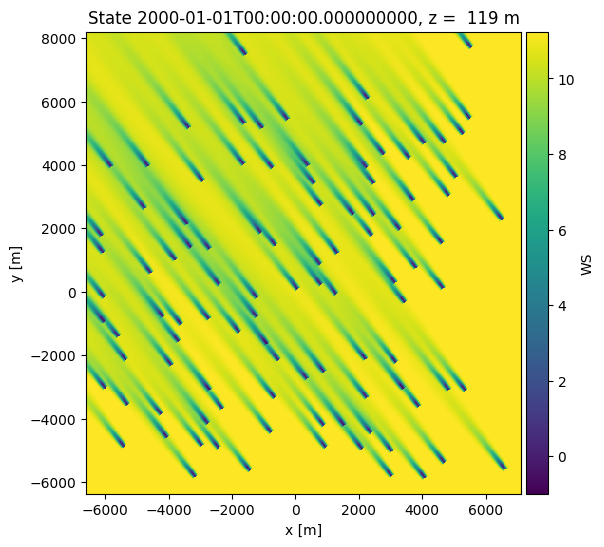
with engine:
farm_results = algo.calc_farm()
o = foxes.output.FlowPlots2D(algo, farm_results)
plot_data = o.get_states_data_xy(FV.WS, resolution=30, states_isel=[0])
g = o.gen_states_fig_xy(plot_data, figsize=(6, 6))
next(g)
plt.show()
Launching local dask cluster..
LocalCluster(25e713cc, 'tcp://127.0.0.1:34387', workers=3, threads=6, memory=15.61 GiB)
Dashboard: http://127.0.0.1:8787/status

LocalClusterEngine: Calculating 5000 states for 100 turbines
LocalClusterEngine: Starting calculation using 3 workers, for 3 states chunks.
LocalClusterEngine: Completed all 3 chunks

LocalClusterEngine: Calculating data at 223533 points for 1 states
LocalClusterEngine: Starting calculation using 3 workers, for 1 states chunks and 23 targets chunks.
LocalClusterEngine: Completed all 23 chunks

Shutting down LocalCluster
Notice the Dashboard link which for this particular choice of engine displays the progress and cluster load during the execution.
Remarks & recommendations
Take the time to think about your engine choice, and its parameters. Your choice might matter a lot for the performance of your run.
In general, all engines accept the parameters
n_procs,chunk_size_states,chunk_size_points(thesingleengine ignores them, though).If
n_procsis not set, the maximal number of processes is applied, according toos.cpu_count()for Python version < 3.13 andos.process_cpu_count()for Python version >= 3.13.If
chunk_size_statesis not set, the number of states is divided byn_procs. This might be non-optimal for small cases.If
chunk_size_pointsis not set and there is more than one states chunk, the full number of points is selected such that there is only one point chunk for each state chunk. If there is only one states chunk, the default points chunk size is the number of points divided byn_procs.In general, for not too small cases, the default
processengine is a good choice for runs on a linux based laptop or a workstation computer, or within Windows WSL.For runs on native Windows, i.e., without WSL, the best engine choices have not been tested. Make sure you try different ones, e.g.
process,multiprocess,dask,numpy,ray, and also vary the parameters.The
mpiengine requires the installation of MPI on the system, for example OpenMPI. Don’t forget to run this as for example for 12 cores bympiexec -n 12 python -m mpi4py.futures run.py, withengine = foxes.Engine.new("mpi", n_procs=12, ...).If you run into memory problems, the best options are to either reduce the number of processes or the chunk sizes.
The
daskengine has additional options, accessible through the dask_pars dictionary parameter, for example the scheduler choice. See API and dask documentation for syntax and more info.The
local_clusteris not always faster than theprocess,multiprocessordaskengines, but offers a more detailed setup. For example, the memory and the number of threads per worker can be modified, if needed.The
numpyandsingleengines are intended for testing and small cases, and also for sequential runs without large point evaluations, or for smallish runs with wake framedyn_wakes.