Layout optimization¶

This example demonstrates some basics about running wind farm optimization tasks with foxes. All optimizations use the iwopy interface in the background (also by Fraunhofer IWES, see link for details).

In the following we invoke the optimization library pymoo which contains a number of very nice genetic algorithm implementations. Within foxes we do that implicitely via the iwopy interface.

These are the required imports for this example:

In [1]:

%matplotlib inline
import numpy as np
import matplotlib.pyplot as plt
from iwopy.interfaces.pymoo import Optimizer_pymoo

import foxes
import foxes.variables as FV
import foxes.utils.geom2d as gm
from foxes.opt.problems.layout import FarmLayoutOptProblem
from foxes.opt.constraints import FarmBoundaryConstraint, MinDistConstraint
from foxes.opt.objectives import MaxFarmPower

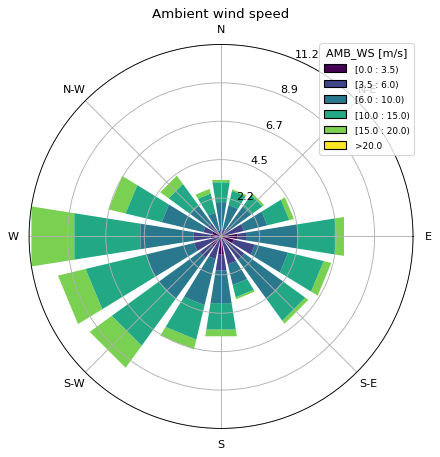
In the following we are tackling the problem of optimizing a wind farm layout for a site near Bremen, Germany. The data of a (coarse) wind rose with 216 states is provided as static data file with name "wind_rose_bremen.csv":

state,wd,ws,weight
0,0.0,3.5,0.00158
1,0.0,6.0,0.00244
2,0.0,8.5,0.00319
3,0.0,12.5,0.0036700002
4,0.0,17.5,0.00042
...

First, let’s create the states object and have a look at the wind rose:

In [2]:

states = foxes.input.states.StatesTable(
    data_source="wind_rose_bremen.csv",
    output_vars=[FV.WS, FV.WD, FV.TI, FV.RHO],
    var2col={FV.WS: "ws", FV.WD: "wd", FV.WEIGHT: "weight"},
    fixed_vars={FV.RHO: 1.225, FV.TI: 0.05},
)

o = foxes.output.StatesRosePlotOutput(states, point=[0., 0., 100.])
fig = o.get_figure(16, FV.AMB_WS, [0, 3.5, 6, 10, 15, 20], figsize=(6, 6))
plt.show()

Next, we need to specify the area within which the turbines are allowed to move during optimization. We use the foxes.utils.geom2d sub-package for that purpose (imported as gm, see above) which allows us to add and subtract polygons, circles, etc.

In [3]:

boundary = \
    gm.ClosedPolygon(np.array(
    [[0, 0], [0, 1200], [1000, 800], [900, -200]], dtype=np.float64)) \
    + gm.ClosedPolygon(np.array(
    [[500, 0], [500, 1500], [1000, 1500], [1000, 0]], dtype=np.float64)) \
    - gm.Circle([-100., -100.], 700)

fig, ax = plt.subplots()
boundary.add_to_figure(ax)
plt.show()

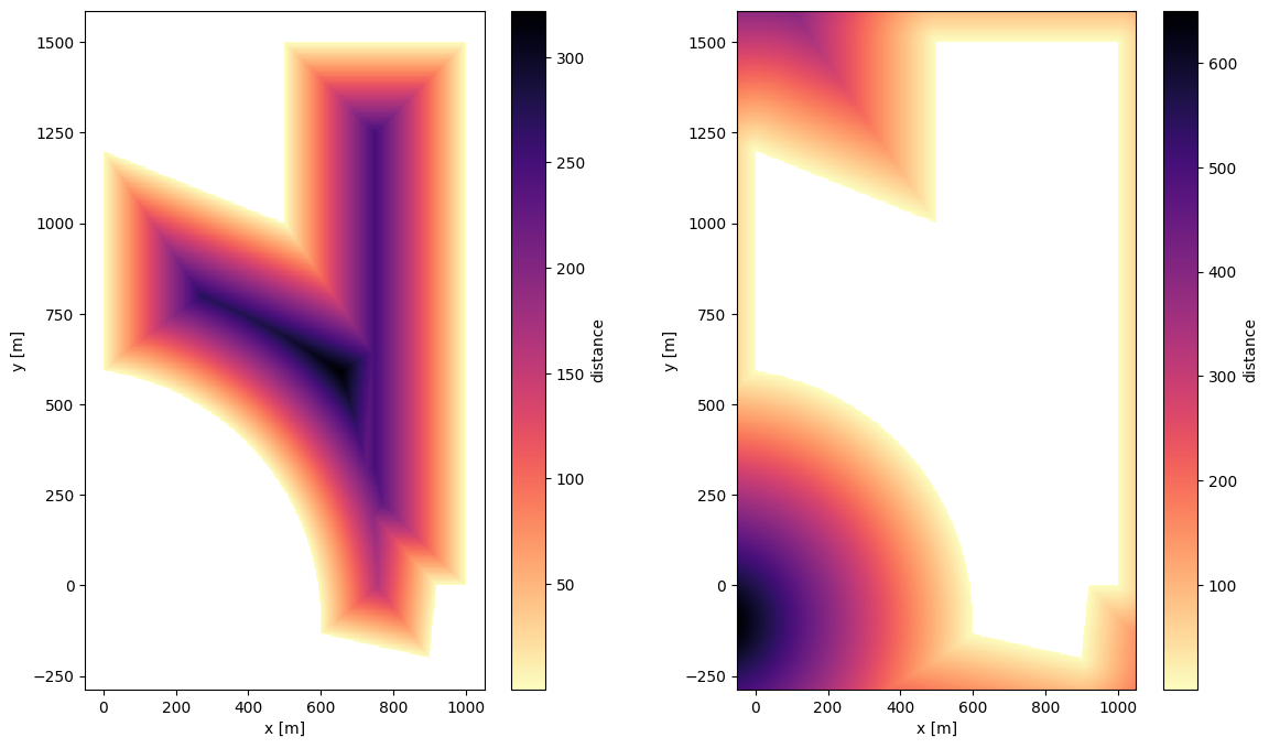
Later on we wish to apply boundary constraints that make sure all turbines are placed within this area geometry. These conditions make use of the minimal distance calculation from each point in question to the boundary. We can check the results by plotting again, now using the fill_mode option:

In [4]:

fig, axs = plt.subplots(1, 2, figsize=(14, 8))
boundary.add_to_figure(axs[0], fill_mode="dist_inside")
boundary.add_to_figure(axs[1], fill_mode="dist_outside")
plt.show()

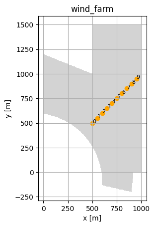
We now setup the model book and a wind farm with 10 turbines in some initial layout, including the boundary:

In [5]:

mbook = foxes.models.ModelBook()

farm = foxes.WindFarm(boundary=boundary)
foxes.input.farm_layout.add_row(
    farm=farm,
    xy_base=np.array([500.0, 500.0]),
    xy_step=np.array([50.0, 50.0]),
    n_turbines=10,
    turbine_models=["layout_opt", "NREL5MW"],
)

ax = foxes.output.FarmLayoutOutput(farm).get_figure()
plt.show()

Turbine 0, T0: layout_opt, NREL5MW
Turbine 1, T1: layout_opt, NREL5MW
Turbine 2, T2: layout_opt, NREL5MW
Turbine 3, T3: layout_opt, NREL5MW
Turbine 4, T4: layout_opt, NREL5MW
Turbine 5, T5: layout_opt, NREL5MW
Turbine 6, T6: layout_opt, NREL5MW
Turbine 7, T7: layout_opt, NREL5MW
Turbine 8, T8: layout_opt, NREL5MW
Turbine 9, T9: layout_opt, NREL5MW

../_images/notebooks_layout_opt_10_1.png

Notice the appearing turbine model layout_opt. This is not part of the model book but will be defined shortly by the optimization problem. In the context of the turbine models it defines where in the model order the optimization variables application should be applied. In our case we are optimizing the (X, Y)-coordinates of the turbines, and they should be updated at the very beginning.

Let’s new define the algorithm and the layout optimization problem. The latter should include boundary constraints and a minimal distance of 2 rotor diameters between turbines. Our objective is the maximization of the total wind farm power:

In [6]:

algo = foxes.algorithms.Downwind(
    mbook,
    farm,
    states=states,
    rotor_model="centre",
    wake_models=["Bastankhah025_linear_k002"],
    wake_frame="rotor_wd",
    partial_wakes_model="auto",
    verbosity=0,
)

problem = FarmLayoutOptProblem("layout_opt", algo)
problem.add_objective(MaxFarmPower(problem))
problem.add_constraint(FarmBoundaryConstraint(problem))
problem.add_constraint(
    MinDistConstraint(problem, min_dist=2., min_dist_unit="D")
)
problem.initialize()

Problem 'layout_opt' (FarmLayoutOptProblem): Initializing
---------------------------------------------------------
  n_vars_int  : 0
  n_vars_float: 20
---------------------------------------------------------
  n_objectives: 1
  n_obj_cmptns: 1
---------------------------------------------------------
  n_constraints: 2
  n_con_cmptns: 55
---------------------------------------------------------

Notice that the two added constraint models imply a total of 55 individual constraint component functions. The wake model choice Bastankhah025 corresponds to the Bastankhah2014 deficit model with parameter sbeta_factor=0.25. This choice switches off the near wake modelling, rendering the model a bit smoother. This is for demonstrational purposes only and not required for running this example.

Next, we setup the optimizer. In our case we use the genetic algorithm GA from pymoo via the iwopy interface, here in vectorized form (flag vectorize=True), with 100 generations (n_max_gen=100) with population size 50 (pop_size=50):

In [7]:

solver = Optimizer_pymoo(
    problem,
    problem_pars=dict(vectorize=True),
    algo_pars=dict(
        type="GA",
        pop_size=50,
        seed=42,
    ),
    setup_pars=dict(),
    term_pars=dict(
        type="default",
        n_max_gen=100,
        ftol=1e-6,
        xtol=1e-3,
    ),
)
solver.initialize()
solver.print_info()

Loading pymoo
pymoo successfully loaded
Initializing Optimizer_pymoo
Selecting sampling: float_random (FloatRandomSampling)
Selecting algorithm: GA (GA)
Selecting termination: default (DefaultSingleObjectiveTermination)

Problem:
--------
  vectorize: True

Algorithm:
----------
  type: GA
  pop_size: 50
  seed: 42

Termination:
------------
  n_max_gen: 100
  ftol: 1e-06
  xtol: 0.001

After all the setup we can now solve the problem:

In [8]:

results = solver.solve()
solver.finalize(results)

print()
print(results)
print(results.problem_results)

=================================================================================
n_gen  |  n_eval  |     cv_min    |     cv_avg    |     f_avg     |     f_min
=================================================================================
     1 |       50 |  4.257950E+02 |  1.094916E+03 |             - |             -
     2 |      100 |  2.589298E+02 |  7.141458E+02 |             - |             -
     3 |      150 |  2.108843E+02 |  5.097684E+02 |             - |             -
     4 |      200 |  2.011586E+02 |  3.869307E+02 |             - |             -
     5 |      250 |  1.250281E+02 |  3.238949E+02 |             - |             -
     6 |      300 |  1.250281E+02 |  2.668302E+02 |             - |             -
     7 |      350 |  1.250281E+02 |  2.500554E+02 |             - |             -
     8 |      400 |  1.011095E+02 |  2.198486E+02 |             - |             -
     9 |      450 |  8.571793E+01 |  1.998508E+02 |             - |             -
    10 |      500 |  8.571793E+01 |  1.775495E+02 |             - |             -
    11 |      550 |  2.695093E+01 |  1.482376E+02 |             - |             -
    12 |      600 |  2.695093E+01 |  1.369663E+02 |             - |             -
    13 |      650 |  2.695093E+01 |  1.255097E+02 |             - |             -
    14 |      700 |  2.461710E+01 |  1.135664E+02 |             - |             -
    15 |      750 |  2.461710E+01 |  1.098324E+02 |             - |             -
    16 |      800 |  2.461710E+01 |  9.266611E+01 |             - |             -
    17 |      850 |  2.446678E+01 |  8.484456E+01 |             - |             -
    18 |      900 |  2.440080E+01 |  7.151751E+01 |             - |             -
    19 |      950 |  2.440080E+01 |  5.917821E+01 |             - |             -
    20 |     1000 |  1.998273E+01 |  4.871628E+01 |             - |             -
    21 |     1050 |  1.019366E+01 |  4.071983E+01 |             - |             -
    22 |     1100 |  6.4405916400 |  3.193676E+01 |             - |             -
    23 |     1150 |  4.9794099827 |  2.349004E+01 |             - |             -
    24 |     1200 |  0.000000E+00 |  1.738912E+01 | -5.632250E-01 | -5.632250E-01
    25 |     1250 |  0.000000E+00 |  1.137290E+01 | -5.629958E-01 | -5.633040E-01
    26 |     1300 |  0.000000E+00 |  5.1859595870 | -5.623456E-01 | -5.633040E-01
    27 |     1350 |  0.000000E+00 |  1.6172307553 | -5.623231E-01 | -5.635398E-01
    28 |     1400 |  0.000000E+00 |  0.0289892170 | -5.623859E-01 | -5.637392E-01
    29 |     1450 |  0.000000E+00 |  0.000000E+00 | -5.630865E-01 | -5.639713E-01
    30 |     1500 |  0.000000E+00 |  0.000000E+00 | -5.636295E-01 | -5.648299E-01
    31 |     1550 |  0.000000E+00 |  0.000000E+00 | -5.639242E-01 | -5.648299E-01
    32 |     1600 |  0.000000E+00 |  0.000000E+00 | -5.642970E-01 | -5.659120E-01
    33 |     1650 |  0.000000E+00 |  0.000000E+00 | -5.647586E-01 | -5.659120E-01
    34 |     1700 |  0.000000E+00 |  0.000000E+00 | -5.651638E-01 | -5.664510E-01
    35 |     1750 |  0.000000E+00 |  0.000000E+00 | -5.656008E-01 | -5.667086E-01
    36 |     1800 |  0.000000E+00 |  0.000000E+00 | -5.660144E-01 | -5.672340E-01
    37 |     1850 |  0.000000E+00 |  0.000000E+00 | -5.664176E-01 | -5.679336E-01
    38 |     1900 |  0.000000E+00 |  0.000000E+00 | -5.668654E-01 | -5.683192E-01
    39 |     1950 |  0.000000E+00 |  0.000000E+00 | -5.672131E-01 | -5.683192E-01
    40 |     2000 |  0.000000E+00 |  0.000000E+00 | -5.675730E-01 | -5.684436E-01
    41 |     2050 |  0.000000E+00 |  0.000000E+00 | -5.679345E-01 | -5.685910E-01
    42 |     2100 |  0.000000E+00 |  0.000000E+00 | -5.682198E-01 | -5.687477E-01
    43 |     2150 |  0.000000E+00 |  0.000000E+00 | -5.684352E-01 | -5.690953E-01
    44 |     2200 |  0.000000E+00 |  0.000000E+00 | -5.686737E-01 | -5.692379E-01
    45 |     2250 |  0.000000E+00 |  0.000000E+00 | -5.688213E-01 | -5.693244E-01
    46 |     2300 |  0.000000E+00 |  0.000000E+00 | -5.690648E-01 | -5.698961E-01
    47 |     2350 |  0.000000E+00 |  0.000000E+00 | -5.693554E-01 | -5.701783E-01
    48 |     2400 |  0.000000E+00 |  0.000000E+00 | -5.696589E-01 | -5.703675E-01
    49 |     2450 |  0.000000E+00 |  0.000000E+00 | -5.699951E-01 | -5.705554E-01
    50 |     2500 |  0.000000E+00 |  0.000000E+00 | -5.702238E-01 | -5.705714E-01
    51 |     2550 |  0.000000E+00 |  0.000000E+00 | -5.704255E-01 | -5.710990E-01
    52 |     2600 |  0.000000E+00 |  0.000000E+00 | -5.706153E-01 | -5.713617E-01
    53 |     2650 |  0.000000E+00 |  0.000000E+00 | -5.708070E-01 | -5.713903E-01
    54 |     2700 |  0.000000E+00 |  0.000000E+00 | -5.709566E-01 | -5.713903E-01
    55 |     2750 |  0.000000E+00 |  0.000000E+00 | -5.711365E-01 | -5.714727E-01
    56 |     2800 |  0.000000E+00 |  0.000000E+00 | -5.712767E-01 | -5.715763E-01
    57 |     2850 |  0.000000E+00 |  0.000000E+00 | -5.713924E-01 | -5.717583E-01
    58 |     2900 |  0.000000E+00 |  0.000000E+00 | -5.715063E-01 | -5.718967E-01
    59 |     2950 |  0.000000E+00 |  0.000000E+00 | -5.716309E-01 | -5.720381E-01
    60 |     3000 |  0.000000E+00 |  0.000000E+00 | -5.717715E-01 | -5.721396E-01
    61 |     3050 |  0.000000E+00 |  0.000000E+00 | -5.718699E-01 | -5.722662E-01
    62 |     3100 |  0.000000E+00 |  0.000000E+00 | -5.719379E-01 | -5.723719E-01
    63 |     3150 |  0.000000E+00 |  0.000000E+00 | -5.720750E-01 | -5.728523E-01
    64 |     3200 |  0.000000E+00 |  0.000000E+00 | -5.721825E-01 | -5.728523E-01
    65 |     3250 |  0.000000E+00 |  0.000000E+00 | -5.723489E-01 | -5.730297E-01
    66 |     3300 |  0.000000E+00 |  0.000000E+00 | -5.724960E-01 | -5.730297E-01
    67 |     3350 |  0.000000E+00 |  0.000000E+00 | -5.726414E-01 | -5.730297E-01
    68 |     3400 |  0.000000E+00 |  0.000000E+00 | -5.728228E-01 | -5.736205E-01
    69 |     3450 |  0.000000E+00 |  0.000000E+00 | -5.729573E-01 | -5.736205E-01
    70 |     3500 |  0.000000E+00 |  0.000000E+00 | -5.730764E-01 | -5.736205E-01
    71 |     3550 |  0.000000E+00 |  0.000000E+00 | -5.732604E-01 | -5.740851E-01
    72 |     3600 |  0.000000E+00 |  0.000000E+00 | -5.734725E-01 | -5.740851E-01
    73 |     3650 |  0.000000E+00 |  0.000000E+00 | -5.736656E-01 | -5.740851E-01
    74 |     3700 |  0.000000E+00 |  0.000000E+00 | -5.738042E-01 | -5.742883E-01
    75 |     3750 |  0.000000E+00 |  0.000000E+00 | -5.739408E-01 | -5.742883E-01
    76 |     3800 |  0.000000E+00 |  0.000000E+00 | -5.740628E-01 | -5.745662E-01
    77 |     3850 |  0.000000E+00 |  0.000000E+00 | -5.742020E-01 | -5.747658E-01
    78 |     3900 |  0.000000E+00 |  0.000000E+00 | -5.743480E-01 | -5.748826E-01
    79 |     3950 |  0.000000E+00 |  0.000000E+00 | -5.745263E-01 | -5.750244E-01
    80 |     4000 |  0.000000E+00 |  0.000000E+00 | -5.746462E-01 | -5.750244E-01
    81 |     4050 |  0.000000E+00 |  0.000000E+00 | -5.747639E-01 | -5.750263E-01
    82 |     4100 |  0.000000E+00 |  0.000000E+00 | -5.748825E-01 | -5.750442E-01
    83 |     4150 |  0.000000E+00 |  0.000000E+00 | -5.749469E-01 | -5.750688E-01
    84 |     4200 |  0.000000E+00 |  0.000000E+00 | -5.750088E-01 | -5.751212E-01
    85 |     4250 |  0.000000E+00 |  0.000000E+00 | -5.750365E-01 | -5.751212E-01
    86 |     4300 |  0.000000E+00 |  0.000000E+00 | -5.750600E-01 | -5.751361E-01
    87 |     4350 |  0.000000E+00 |  0.000000E+00 | -5.750885E-01 | -5.752174E-01
    88 |     4400 |  0.000000E+00 |  0.000000E+00 | -5.751208E-01 | -5.752654E-01
    89 |     4450 |  0.000000E+00 |  0.000000E+00 | -5.751561E-01 | -5.752717E-01
    90 |     4500 |  0.000000E+00 |  0.000000E+00 | -5.751994E-01 | -5.752956E-01
    91 |     4550 |  0.000000E+00 |  0.000000E+00 | -5.752418E-01 | -5.753591E-01
    92 |     4600 |  0.000000E+00 |  0.000000E+00 | -5.752717E-01 | -5.755239E-01
    93 |     4650 |  0.000000E+00 |  0.000000E+00 | -5.753058E-01 | -5.755383E-01
    94 |     4700 |  0.000000E+00 |  0.000000E+00 | -5.753560E-01 | -5.755434E-01
    95 |     4750 |  0.000000E+00 |  0.000000E+00 | -5.754149E-01 | -5.755434E-01
    96 |     4800 |  0.000000E+00 |  0.000000E+00 | -5.754853E-01 | -5.756107E-01
    97 |     4850 |  0.000000E+00 |  0.000000E+00 | -5.755318E-01 | -5.756331E-01
    98 |     4900 |  0.000000E+00 |  0.000000E+00 | -5.755540E-01 | -5.756656E-01
    99 |     4950 |  0.000000E+00 |  0.000000E+00 | -5.755761E-01 | -5.756656E-01
   100 |     5000 |  0.000000E+00 |  0.000000E+00 | -5.756008E-01 | -5.756656E-01


Optimizer_pymoo: Optimization run finished
  Success: True
  Best maximize_power = 28783.277672267686

Results problem 'layout_opt':
------------------------------
  Float variables:
    0: X_0000 = 6.114235e+02
    1: Y_0000 = -1.311872e+02
    2: X_0001 = 1.197274e-01
    3: Y_0001 = 6.544626e+02
    4: X_0002 = 9.998818e+02
    5: Y_0002 = 1.087410e+03
    6: X_0003 = 9.932613e+02
    7: Y_0003 = 1.498619e+03
    8: X_0004 = 9.951248e+02
    9: Y_0004 = 4.494226e+02
    10: X_0005 = 1.365731e+00
    11: Y_0005 = 1.180728e+03
    12: X_0006 = 4.168690e+02
    13: Y_0006 = 3.726276e+02
    14: X_0007 = 5.468598e+02
    15: Y_0007 = 9.232537e+02
    16: X_0008 = 9.999757e+02
    17: Y_0008 = 1.507834e+00
    18: X_0009 = 5.017820e+02
    19: Y_0009 = 1.495002e+03
------------------------------
  Objectives:
    0: maximize_power = 2.878328e+04
------------------------------
  Constraints:
    0: boundary_0000 = -4.573154e+00
    1: boundary_0001 = -1.197274e-01
    2: boundary_0002 = -1.182467e-01
    3: boundary_0003 = -1.381264e+00
    4: boundary_0004 = -4.875224e+00
    5: boundary_0005 = -1.365731e+00
    6: boundary_0006 = -3.787956e-01
    7: boundary_0007 = -5.385391e+01
    8: boundary_0008 = -2.426929e-02
    9: boundary_0009 = -1.781952e+00
    10: dist_0_1      = -7.434586e+02
    11: dist_0_2      = -1.027015e+03
    12: dist_0_3      = -1.421938e+03
    13: dist_0_4      = -4.439414e+02
    14: dist_0_5      = -1.194822e+03
    15: dist_0_6      = -2.880748e+02
    16: dist_0_7      = -8.044156e+02
    17: dist_0_8      = -1.585859e+02
    18: dist_0_9      = -1.377881e+03
    19: dist_1_2      = -8.374803e+02
    20: dist_1_3      = -1.051430e+03
    21: dist_1_4      = -7.639116e+02
    22: dist_1_5      = -2.742672e+02
    23: dist_1_6      = -2.511013e+02
    24: dist_1_7      = -3.572399e+02
    25: dist_1_8      = -9.421784e+02
    26: dist_1_9      = -7.268625e+02
    27: dist_2_3      = -1.592622e+02
    28: dist_2_4      = -3.860049e+02
    29: dist_2_5      = -7.508672e+02
    30: dist_2_6      = -6.703977e+02
    31: dist_2_7      = -2.298466e+02
    32: dist_2_8      = -8.339020e+02
    33: dist_2_9      = -3.916108e+02
    34: dist_3_4      = -7.971977e+02
    35: dist_3_5      = -7.895907e+02
    36: dist_3_6      = -1.012944e+03
    37: dist_3_7      = -4.762303e+02
    38: dist_3_8      = -1.245126e+03
    39: dist_3_9      = -2.394927e+02
    40: dist_4_5      = -9.818416e+02
    41: dist_4_6      = -3.313328e+02
    42: dist_4_7      = -4.002709e+02
    43: dist_4_8      = -1.959411e+02
    44: dist_4_9      = -9.041244e+02
    45: dist_5_6      = -6.566637e+02
    46: dist_5_7      = -3.512055e+02
    47: dist_5_8      = -1.293245e+03
    48: dist_5_9      = -3.389183e+02
    49: dist_6_7      = -3.137620e+02
    50: dist_6_8      = -4.391898e+02
    51: dist_6_9      = -8.735820e+02
    52: dist_7_8      = -7.750976e+02
    53: dist_7_9      = -3.215227e+02
    54: dist_8_9      = -1.322396e+03
------------------------------
  Success: True
------------------------------

<xarray.Dataset>
Dimensions:    (state: 216, turbine: 10)
Coordinates:
  * state      (state) int64 0 1 2 3 4 5 6 7 ... 208 209 210 211 212 213 214 215
Dimensions without coordinates: turbine
Data variables: (12/25)
    AMB_CT     (state, turbine) float64 0.995 0.995 0.995 ... 0.081 0.081 0.081
    AMB_P      (state, turbine) float64 109.1 109.1 109.1 ... 5e+03 5e+03 5e+03
    AMB_REWS   (state, turbine) float64 3.5 3.5 3.5 3.5 ... 20.0 20.0 20.0 20.0
    AMB_REWS2  (state, turbine) float64 3.5 3.5 3.5 3.5 ... 20.0 20.0 20.0 20.0
    AMB_REWS3  (state, turbine) float64 3.5 3.5 3.5 3.5 ... 20.0 20.0 20.0 20.0
    AMB_RHO    (state, turbine) float64 1.225 1.225 1.225 ... 1.225 1.225 1.225
    ...         ...
    X          (state, turbine) float64 611.4 0.1197 999.9 ... 546.9 1e+03 501.8
    Y          (state, turbine) float64 -131.2 654.5 ... 1.508 1.495e+03
    YAW        (state, turbine) float64 0.0 0.0 0.0 0.0 ... 350.0 350.0 350.0
    order      (state, turbine) int64 3 9 5 2 7 1 4 6 8 0 ... 3 5 2 7 1 6 4 8 0
    weight     (state, turbine) float64 0.00158 0.00158 ... 0.00013 0.00013
    tname      (turbine) <U2 'T0' 'T1' 'T2' 'T3' 'T4' 'T5' 'T6' 'T7' 'T8' 'T9'

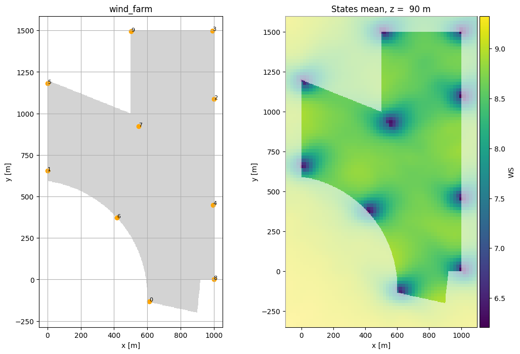
This visualizes the results, once the layout and once the mean wind speed over all wind rose states:

In [9]:

fig, axs = plt.subplots(1, 2, figsize=(12, 8))

foxes.output.FarmLayoutOutput(farm).get_figure(fig=fig, ax=axs[0])

o = foxes.output.FlowPlots2D(algo, results.problem_results)
p_min = np.array([-100.0, -350.0])
p_max = np.array([1100.0, 1600.0])
fig = o.get_mean_fig_xy("WS", resolution=20, fig=fig, ax=axs[1],
    xmin=p_min[0], xmax=p_max[0], ymin=p_min[1], ymax=p_max[1])
dpars = dict(alpha=0.6, zorder=10, p_min=p_min, p_max=p_max)
farm.boundary.add_to_figure(
    axs[1], fill_mode="outside_white", pars_distance=dpars
)

plt.show()

../_images/notebooks_layout_opt_18_0.png

Note that the optimization can also be run using a DaskRunner, i.e., optionally in parallel on a (local) cluster. For that invoke the runner parameter when creating the problem within awith block and solve the problem as before:

with foxes.utils.runners.DaskRunner(scheduler="distributed") as runner:

    problem = FarmLayoutOptProblem("layout_opt", algo, runner=runner)
    ...
    solver = ...
    ...
    results = solver.solve()

Anything within the with block will then be calculated using the runner. This includes the output figures, if they appear there as well.