Heterogeneous flow
The best way to run foxes calculations on heterogeneous background flow fields is by providing them in netCDF format. The following coordinates are supported (can be None if not present):
A state coordinate, e.g.
Time(expected by default) orstate, or similarA height coordinate, e.g.
height(expected by default) orh, or similarA
ycoordinate, e.g.UTMY(expected by default) ory, or similarA
xcoordinate, e.g.UTMX(expected by default) orx, or similar
The file may contain any kind of foxes variables as data fields, e.g.:
Wind speed data, e.g.
WS(expected by default, if claimed as output variable),wsor similarWind direction data, e.g.
WD(expected by default, if claimed as output variable),wdor similarTurbulence intensity data, e.g.
TI(expected by default, if claimed as output variable),tior similarAir density data, e.g.
RHO(expected by default, if claimed as output variable),rhoor similar
All data must depend on the state coordinate, and may depend on the others.
These are the required imports for this example:
%matplotlib inline
import matplotlib.pyplot as plt
import numpy as np

import foxes
import foxes.variables as FV
/home/runner/work/foxes/foxes/foxes/core/engine.py:4: TqdmExperimentalWarning: Using `tqdm.autonotebook.tqdm` in notebook mode. Use `tqdm.tqdm` instead to force console mode (e.g. in jupyter console)
  from tqdm.autonotebook import tqdm
For parallelization we will use the following engine:
engine = foxes.Engine.new("process")
One very simple example for netCDF type data is provided in the static data, under the name wind_rotation.nc. It contains two states, two heights, and simple 2 x 2 horizontal data that describes identical wind speeds at all four corner points associated with different wind direction values. It can be loaded as follows:
states = foxes.input.states.FieldData(
    data_source="wind_rotation.nc",
    states_coord="state",
    x_coord="x",
    y_coord="y",
    h_coord="h",
    time_format=None,
    output_vars=[FV.WS, FV.WD, FV.TI, FV.RHO],
    var2ncvar={FV.WS: "ws", FV.WD: "wd"},
    fixed_vars={FV.RHO: 1.225, FV.TI: 0.1},
    load_mode="preload",
    bounds_extra_space=1000,
    interp_pars=dict(bounds_error=False),
)
The bounds_extra_space parameter is here set to 1000 meters. Alternatively, distances can be specified as multiples of the rotor diameter as string, e.g., 2D. If not None this cuts the input data spatially to the specified extension of the wind farm boundary area.
Note that it is recommended that the states object should be created outside the Engine context when working with NetCFD input.
Now back to our example. Let’s place a simple 3 x 3 grid wind farm inside the data domain, which is a rectangle between (0, 0) and (2500, 2500):
farm = foxes.WindFarm()
foxes.input.farm_layout.add_grid(
    farm,
    xy_base=np.array([500.0, 500.0]),
    step_vectors=np.array([[500.0, 0], [0, 500.0]]),
    steps=(3, 3),
    turbine_models=["NREL5MW"],
    verbosity=0,
)
The streamline following wakes are realized by selecting a wake frame that is an instance of foxes.models.wake_frames.Streamlines2D, e.g. the model streamlines_100 in the model book. This model has a streamline step size of 100 m. Additionally we define a maximal wake length of 3 km for this example:
algo = foxes.algorithms.Downwind(
    farm,
    states,
    rotor_model="grid16",
    wake_models=["Jensen_linear_k007"],
    wake_frame="streamlines_100",
    max_wake_length_km=3.0,
    verbosity=0,
)
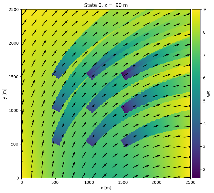
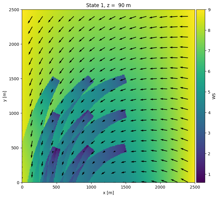
We run the algorithm, once explicitely for calculating the wind farm data, and once implicitely when creating horizontal flow plots:
with engine:
    farm_results = algo.calc_farm()

    fr = farm_results.to_dataframe()
    print(fr[[FV.WD, FV.AMB_REWS, FV.REWS, FV.AMB_P, FV.P]])

    o = foxes.output.FlowPlots2D(algo, farm_results)
    plot_data = o.get_states_data_xy(
        FV.WS,
        resolution=10,
        xmin=0,
        xmax=2500,
        ymin=0,
        ymax=2500,
    )

for fig in o.gen_states_fig_xy(
    plot_data,
    figsize=(8, 8),
    quiver_pars=dict(angles="xy", scale_units="xy", scale=0.07),
    quiver_n=15,
):
    plt.show()
    plt.close(fig)
ProcessEngine: Calculating 2 states for 9 turbines
ProcessEngine: Starting calculation using 3 workers, for 2 states chunks.
ProcessEngine: Completed all 2 chunks

                       WD  AMB_REWS      REWS        AMB_P            P
state turbine
0     0        201.158095  7.491089  7.491089  1474.211485  1474.211485
      1        208.044995  7.673386  7.673386  1580.523149  1580.523149
      2        214.523994  7.960601  7.960601  1748.171150  1748.171150
      3        218.242347  6.867298  6.867298  1127.597890  1127.597890
      4        222.297881  7.283373  7.283373  1352.715592  1352.715592
      5        225.899315  7.731909  6.812258  1614.607094  1102.830918
      6        236.751305  6.932726  6.932726  1156.958724  1156.958724
      7        237.139686  7.375640  7.375640  1406.547921  1406.547921
      8        237.484050  7.818854  7.818854  1665.346938  1665.346938
1     0         20.311353  6.703701  5.738961  1054.871497   651.260571
      1         26.259090  6.995899  5.942901  1185.898437   719.019801
      2         31.676969  7.357075  7.357075  1396.122885  1396.122885
      3         44.537114  5.352448  5.352448   521.748601   521.748601
      4         47.447854  5.960030  5.960030   724.421355   724.421355
      5         49.815210  6.580130  6.580130   998.581133   998.581133
      6         75.462890  5.352661  5.352661   521.621885   521.621885
      7         72.552150  5.960214  5.960214   724.363441   724.363441
      8         70.184794  6.580285  6.580285   998.552613   998.552613
ProcessEngine: Calculating data at 63001 points for 2 states
ProcessEngine: Starting calculation using 3 workers, for 2 states chunks and 3 targets chunks.
ProcessEngine: Completed all 6 chunks