Turbine operation flags
This example demonstrates how to run a wind farm simulation with given operational flags, that indicate if turbines are switched on or off at each state. There is more than one way for achieving this within foxes, but here we will make use of the OpFlagController which was specifically added for this purpose.
These are the imports that we will need:
%matplotlib inline
import numpy as np
import pandas as pd
import xarray as xr
import matplotlib.pyplot as plt

import foxes
import foxes.variables as FV
import foxes.constants as FC
/home/runner/work/foxes/foxes/foxes/core/engine.py:4: TqdmExperimentalWarning: Using `tqdm.autonotebook.tqdm` in notebook mode. Use `tqdm.tqdm` instead to force console mode (e.g. in jupyter console)
  from tqdm.autonotebook import tqdm
This example uses the default engine:
engine = foxes.Engine.new("default")
We first generate the input data, starting with three simple wind states:
sdata = pd.DataFrame(
    {
        FV.WS: [10, 10, 10],
        FV.WD: [270, 270, 90],
    }
)
sdata.index.name = FC.STATE
sdata
| WS | WD | |
|---|---|---|
| state | ||
| 0 | 10 | 270 |
| 1 | 10 | 270 |
| 2 | 10 | 90 |
The spatially uniform states based on this data are created by
states = foxes.input.states.StatesTable(
    sdata,
    output_vars=[FV.WS, FV.WD, FV.TI, FV.RHO],
    fixed_vars={FV.TI: 0.05, FV.RHO: 1.225},
)
We consider a simple row of turbines as our wind farm:
farm = foxes.WindFarm()
foxes.input.farm_layout.add_row(
    farm=farm,
    xy_base=[0.0, 0.0],
    xy_step=[800.0, 0.0],
    n_turbines=3,
    turbine_models=["DTU10MW"],
    verbosity=0,
)
Now let’s create the operational flag for the 3 states and 3 turbines:
odata = xr.Dataset(
    {
        FV.OPERATING: (
            (FC.STATE, FC.TURBINE),
            np.array(
                [
                    [1, 1, 1],
                    [0, 1, 1],
                    [0, 0, 1],
                ],
                dtype=bool,
            ),
        )
    }
)
odata[FV.OPERATING].values
array([[ True,  True,  True],
       [False,  True,  True],
       [False, False,  True]])
We now create the OpFlagController based on this data, and select it when creating the algorithm object:
mbook = foxes.ModelBook()
mbook.farm_controllers["op_cntrl"] = foxes.models.farm_controllers.OpFlagController(
    odata
)
algo = foxes.algorithms.Downwind(
    farm,
    states,
    wake_models=["Bastankhah2014_linear_lim_k004"],
    farm_controller="op_cntrl",
    mbook=mbook,
)
We can now calculate the farm results:
with engine:
    farm_results = algo.calc_farm()
farm_results.to_dataframe()[[FV.WD, FV.AMB_REWS, FV.REWS, FV.CT, FV.P, FV.OPERATING]]
Initializing model 'StatesTable'

Initializing algorithm 'Downwind'

------------------------------------------------------------
  Algorithm: Downwind
  Running Downwind: calc_farm
------------------------------------------------------------
  n_states : 3
  n_turbines: 3
------------------------------------------------------------
  states    : StatesTable()
  rotor     : CentreRotor()
  controller: OpFlagController()
  deflection: NoDeflection()
  wake frame: RotorWD()
  wake lngth: None
------------------------------------------------------------
  wakes:
    0) Bastankhah2014_linear_lim_k004: Bastankhah2014(ws_linear_lim, induction=Madsen, k=0.04)
------------------------------------------------------------
  partial wakes:
    0) Bastankhah2014_linear_lim_k004: axiwake6, PartialAxiwake(n=6)
------------------------------------------------------------
  turbine models:
    0) DTU10MW: PCtFile(D=178.3, H=119.0, P_nominal=10000.0, P_unit=kW, rho=1.225, var_ws_ct=REWS2, var_ws_P=REWS3)
------------------------------------------------------------


--------------------------------------------------
  Model oder
--------------------------------------------------
00) op_cntrl
01) InitFarmData
02) centre
03) op_cntrl
  03.0) Post-rotor: DTU10MW
04) SetAmbFarmResults
05) FarmWakesCalculation
06) ReorderFarmOutput
--------------------------------------------------


Input data:

 <xarray.Dataset> Size: 134B
Dimensions:           (state: 3, StatesTable_vars: 2, turbine: 3, tmodels: 1)
Coordinates:
  * state             (state) int64 24B 0 1 2
  * StatesTable_vars  (StatesTable_vars) <U2 16B 'WD' 'WS'
  * tmodels           (tmodels) <U7 28B 'DTU10MW'
Dimensions without coordinates: turbine
Data variables:
    StatesTable_data  (state, StatesTable_vars) int64 48B 270 10 270 10 90 10
    tmodel_sels       (state, turbine, tmodels) bool 9B True True ... False True
    operating         (state, turbine) bool 9B True True True ... False True


Farm variables: AMB_CT, AMB_P, AMB_REWS, AMB_REWS2, AMB_REWS3, AMB_RHO, AMB_TI, AMB_WD, AMB_YAW, CT, D, H, P, REWS, REWS2, REWS3, RHO, TI, WD, X, Y, YAW, operating, order, order_inv, order_ssel, weight

Output variables: AMB_CT, AMB_P, AMB_REWS, AMB_REWS2, AMB_REWS3, AMB_RHO, AMB_TI, AMB_WD, AMB_YAW, CT, D, H, P, REWS, REWS2, REWS3, RHO, TI, WD, X, Y, YAW, operating, order, order_inv, order_ssel, weight
DefaultEngine: Selecting engine 'single'
SingleChunkEngine: Calculating 3 states for 3 turbines
SingleChunkEngine: Starting calculation using a single worker.
SingleChunkEngine: Completed all 1 chunks
| WD | AMB_REWS | REWS | CT | P | operating | ||
|---|---|---|---|---|---|---|---|
| state | turbine | ||||||
| 0 | 0 | 270.0 | 10.0 | 10.000000 | 0.814000 | 7286.500000 | True |
| 1 | 270.0 | 10.0 | 7.637441 | 0.829953 | 3286.710475 | True | |
| 2 | 270.0 | 10.0 | 6.958701 | 0.859900 | 2465.899141 | True | |
| 1 | 0 | 270.0 | 10.0 | 10.000000 | 0.000000 | 0.000000 | False |
| 1 | 270.0 | 10.0 | 10.000000 | 0.814000 | 7286.500000 | True | |
| 2 | 270.0 | 10.0 | 7.637441 | 0.829953 | 3286.710475 | True | |
| 2 | 0 | 90.0 | 10.0 | 8.778113 | 0.000000 | 0.000000 | False |
| 1 | 90.0 | 10.0 | 7.637441 | 0.000000 | 0.000000 | False | |
| 2 | 90.0 | 10.0 | 10.000000 | 0.814000 | 7286.500000 | True |
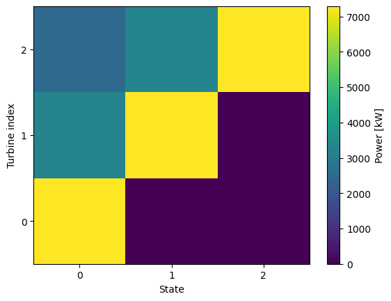
Indeed the power and ct values are zero for non-operating turbines. In fact the turbine type and all other turbine models are not evaluated at all for those turbines. The non-operating values for the variables are zero for FV.P and FV.CT and np.nan for the rest. This choices can be overloaded by passing a dictionary for the parameter non_op_values in the constructor of the OpFlagController class.
One way of visualizing the power pattern for all states and turbines is the StateTurbineMap, indicating the zero power results for the switched-off turbines:
o = foxes.output.StateTurbineMap(farm_results)
ax = o.plot_map(FV.P, cbar_label="Power [kW]")
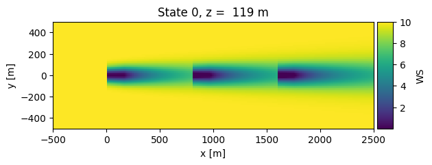
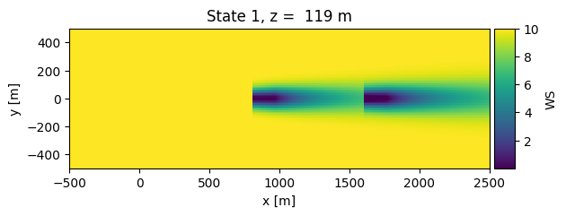
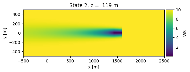
Finally, let’s look at the flow fields of the three states. The non-operating turbines do not contribute to the wakes:
with engine:
    o = foxes.output.FlowPlots2D(algo, farm_results)
    plot_data = o.get_states_data_xy(
        FV.WS, resolution=10, xmin=-500, xmax=2500, verbosity=0
    )

for fig in o.gen_states_fig_xy(plot_data):
    plt.show()
DefaultEngine: Selecting engine 'process'
ProcessEngine: Calculating data at 30401 points for 3 states
ProcessEngine: Starting calculation using 3 workers, for 3 states chunks and 3 targets chunks.
ProcessEngine: Completed all 9 chunks