Wind sector management¶

In this example we switch off, derate or boost turbines according to wind conditions. Here are our imports:

%matplotlib inline
import pandas as pd
import matplotlib.pyplot as plt

import foxes
import foxes.variables as FV

/home/runner/work/foxes/foxes/foxes/core/engine.py:4: TqdmExperimentalWarning: Using `tqdm.autonotebook.tqdm` in notebook mode. Use `tqdm.tqdm` instead to force console mode (e.g. in jupyter console)
  from tqdm.autonotebook import tqdm

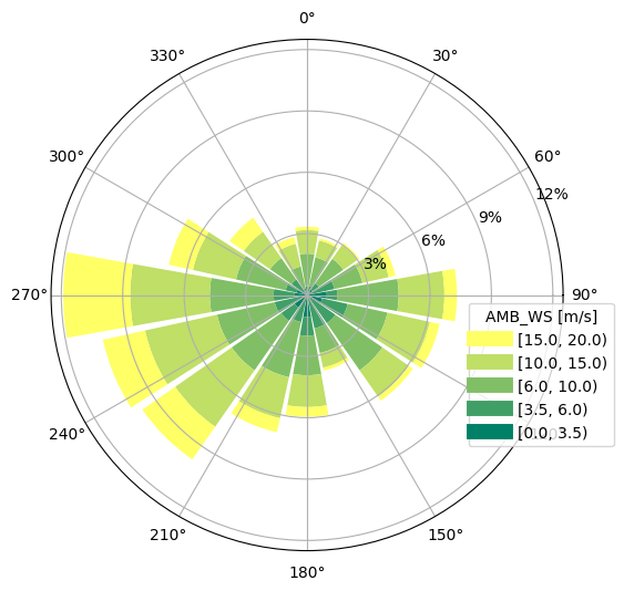
Our wind conditions come from the Bremen wind rose (part of foxes’ static data):

states = foxes.input.states.StatesTable(
    data_source="wind_rose_bremen.csv",
    output_vars=[FV.WS, FV.WD, FV.TI, FV.RHO],
    var2col={FV.WS: "ws", FV.WD: "wd", FV.WEIGHT: "weight"},
    fixed_vars={FV.RHO: 1.225, FV.TI: 0.05},
)

o = foxes.output.StatesRosePlotOutput(states, point=[0.0, 0.0, 100.0])
o.get_figure(16, FV.AMB_WS, [0, 3.5, 6, 10, 15, 20], figsize=(6, 6))
plt.show()

DefaultEngine: Selecting engine 'single'
SingleChunkEngine: Calculating 216 states for 1 turbines
SingleChunkEngine: Starting calculation using a single worker.
SingleChunkEngine: Completed all 1 chunks

../_images/ab29900792f59c7384e3c0c041704d4084aa0391dac95d547a6eb8e8b37df88d.png

The rules of wind sector management can either be given by a pandas readable file like .csv, or directly by a pandas.DataFrame object. Here we are persuing the latter option, for a wind farm that consists of two turbines, labelled T0 and T1, where turbine T1 is located east of turbine T0. This creates the table of rules:

rules = pd.DataFrame(columns=["tname", "WD_min", "WD_max", "WS_min", "WS_max", "MAXP"])
rules.index.name = "rule"
rules.loc[0] = ["T0", 170, 191, 3, 15, 500]
rules.loc[1] = ["T0", 250, 290, 9, 99, 0]
rules.loc[2] = ["T0", 340, 50, 0, 99, 0]
rules.loc[3] = ["T1", 70, 110, 3, 99, 0]
rules.loc[4] = ["T1", 250, 290, 9, 99, 6000]
rules

	tname	WD_min	WD_max	WS_min	WS_max	MAXP
rule
0	T0	170	191	3	15	500
1	T0	250	290	9	99	0
2	T0	340	50	0	99	0
3	T1	70	110	3	99	0
4	T1	250	290	9	99	6000

Note that we can add multiple rules per turbine. Additional conditions on ranges of other variables can be added in addition to WD and WS by simply adding the corresponsing columns with min and max data.

The final column MAXP defines the values of the state-turbine variable that should be set if the current wind conditions fulfill the formulated range conditions. It is possible to add more variables by adding the corresponding columns to the table.

Let’s setup the model book, featuring the SectorManagement turbine model based on the above rules:

mbook = foxes.models.ModelBook()
ttype = foxes.models.turbine_types.PCtFile("NREL-5MW-D126-H90.csv")
mbook.turbine_types[ttype.name] = ttype

mbook.turbine_models["sector_rules"] = foxes.models.turbine_models.SectorManagement(
    data_source=rules,
    col_tnames="tname",
    range_vars=[FV.WD, FV.REWS],
    target_vars=[FV.MAX_P],
    colmap={"REWS_min": "WS_min", "REWS_max": "WS_max"},
)

Due to the stated ``range_varsthe model will look for columnsWD_min, WD_max, REWS_min, REWS_max. The latter two have slightly different names in the DataFrame, hence the entries in the colmap` dict. Notice that also target variable names could be mapped to other column names, if needed.

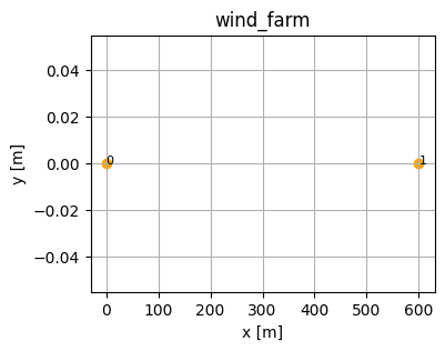
Now we create the wind farm with the two wind turbines in west-east orientation:

farm = foxes.WindFarm()
foxes.input.farm_layout.add_row(
    farm=farm,
    xy_base=[0.0, 0.0],
    xy_step=[600.0, 0.0],
    n_turbines=2,
    turbine_models=[ttype.name, "sector_rules", "PMask"],
)

ax = foxes.output.FarmLayoutOutput(farm).get_figure(figsize=(4, 3))
plt.show(ax.get_figure())

Turbine 0, T0: xy=(0.00, 0.00), NREL-5MW, sector_rules, PMask
Turbine 1, T1: xy=(600.00, 0.00), NREL-5MW, sector_rules, PMask

../_images/02b37ae527a23e5820be030c471603a14fccb6f3bad4014527ab4d304ac2ae28.png

The turbine model PMask was added in order to evaluate the variable MAXP that was set by the sector_rules model. It is responsible for switching off, derating or boosting turbines, cf. example Power mask.

Now let’s create an algorithm object and run the case:

algo = foxes.algorithms.Downwind(
    farm,
    states=states,
    rotor_model="centre",
    wake_models=["Bastankhah2014_linear_k002"],
    mbook=mbook,
    verbosity=0,
)

farm_results = algo.calc_farm()

DefaultEngine: Selecting engine 'single'
SingleChunkEngine: Calculating 216 states for 2 turbines
SingleChunkEngine: Starting calculation using a single worker.
SingleChunkEngine: Completed all 1 chunks

The effect of the rules is best visualized in rose plots for the two turbines:

fig = plt.figure(figsize=(12, 4))
ax1 = fig.add_subplot(121, polar=True)
ax2 = fig.add_subplot(122, polar=True)

o = foxes.output.RosePlotOutput(farm_results)
o.get_figure(
    16,
    FV.P,
    [100, 1000, 2000, 4000, 5001, 7000],
    turbine=0,
    title="Power turbine 0",
    fig=fig,
    ax=ax1,
)

o = foxes.output.RosePlotOutput(farm_results)
o.get_figure(
    16,
    FV.P,
    [100, 1000, 2000, 4000, 5001, 7000],
    turbine=1,
    title="Power turbine 1",
    fig=fig,
    ax=ax2,
)
plt.show()

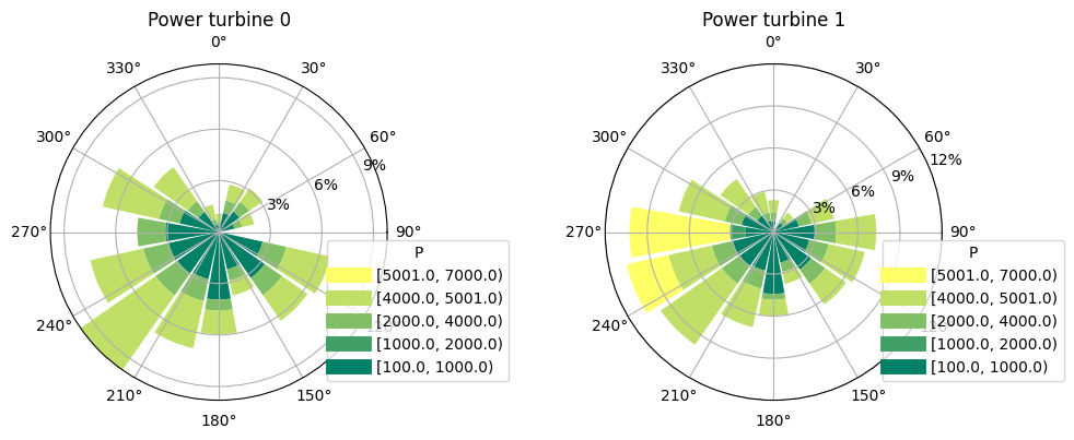
../_images/e9b70b1aadc25b3b809a9b69c436e09df9df092312571bc74e97162fb85e07c8.png

The wind sector management has the following effects (compare to the rules table above):

Turbine 0 switches off at high wind speeds for westerly wind directions
Turbine 1 is boosted for such winds
Turbine 1 switches off completely for wind from east
Turbine 0 is derated for wind from south
Turbine 0 switches off for wind from north