Multi-height wind data
In this example we explore the calculation of multi-height wind data, as for example obtained from WRF results or downloaded from the NEWA website at a single point.
Here we will use the static data file WRF-Timeseries-3000.nc that is part of the foxes static data.
The time coordinate marks one month in 10 minute steps, and the wind speed (WS), wind direction (WD) and turbulent intensity (TI) are provided at 8 heights between 50 and 500 m. The air density (RHO) does not have height dependency but varies with time. The detailed data structure will be displayed below.
The basic assumption of this example is that we can calculate our wind farm results based on this data, i.e., that the horizontal variation can be neglected (for completely heterogeneous inflow data, see the corresponding example).
These are the imports for this example:
%matplotlib inline
import matplotlib.pyplot as plt
from xarray import open_dataset

import foxes
import foxes.variables as FV
/home/runner/work/foxes/foxes/foxes/core/engine.py:4: TqdmExperimentalWarning: Using `tqdm.autonotebook.tqdm` in notebook mode. Use `tqdm.tqdm` instead to force console mode (e.g. in jupyter console)
  from tqdm.autonotebook import tqdm
We use the default engine for the computations in this example:
engine = foxes.Engine.new("default")
First, we setup the model book and the wind farm. We choose 5 turbines in a row:
# create wind farm, a single row of turbines:
farm = foxes.WindFarm()
foxes.input.farm_layout.add_row(
    farm=farm,
    xy_base=[0.0, 0.0],
    xy_step=[600.0, 0.0],
    n_turbines=5,
    turbine_models=["NREL5MW"],
    H=200.0,
    verbosity=0,
)

ax = foxes.output.FarmLayoutOutput(farm).get_figure(figsize=(5, 3))
plt.show()
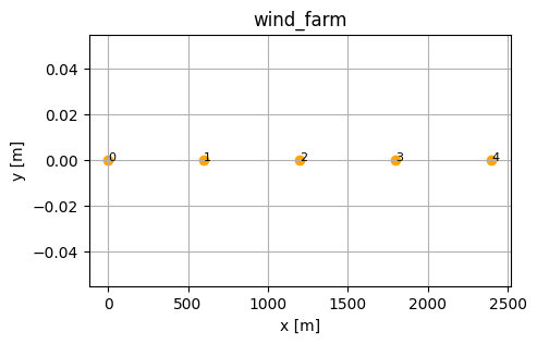
Note that we manually change the hub height from 90 m to 200 m here. Next, we create the states based on the static data file WRF-Timeseries-3000.nc:
# This is what the nc file looks like:
fpath = foxes.StaticData().get_file_path(foxes.STATES, "WRF-Timeseries-3000.nc")
with open_dataset(fpath) as ds:
    print(ds)
<xarray.Dataset> Size: 528kB
Dimensions:  (Time: 3000, height: 8)
Coordinates:
  * Time     (Time) <U19 228kB '2009-01-01 00:00:00' ... '2009-01-21 19:50:00'
  * height   (height) float32 32B 50.0 75.0 90.0 100.0 150.0 200.0 250.0 500.0
Data variables:
    ws       (Time, height) float32 96kB ...
    wd       (Time, height) float32 96kB ...
    ti       (Time, height) float32 96kB ...
    rho      (Time) float32 12kB ...
Now let’s create the corresponding states object:
states = foxes.input.states.MultiHeightNCTimeseries(
    data_source="WRF-Timeseries-3000.nc",
    time_coord="Time",
    h_coord="height",
    output_vars=[FV.WS, FV.WD, FV.TI, FV.RHO],
    var2col={FV.WS: "ws", FV.WD: "wd", FV.TI: "ti", FV.RHO: "rho"},
)

with engine:
    o = foxes.output.StatesRosePlotOutput(states, point=[0.0, 0.0, 100.0])
o.get_figure(16, FV.AMB_WS, [0, 3.5, 6, 10, 15, 20], figsize=(6, 6))
plt.show()
DefaultEngine: Selecting engine 'single'
SingleChunkEngine: Calculating 3000 states for 1 turbines
SingleChunkEngine: Starting calculation using a single worker.
SingleChunkEngine: Completed all 1 chunks
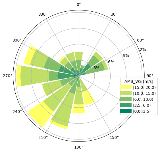
Note how the var2col option offers a mapping from the expected to the actual column names, if needed.
Let’s next setup our algorithm. Notice that we include the z-sensitive rotor model level10, with 10 points on a vertical line (also the grid models would be an option). The partial wakes choice None represents default settings for all wake models. It is important that we do not select rotor_points together with the level10 rotor, since averaging over a vertical line of points does not make much sense.
algo = foxes.algorithms.Downwind(
    farm,
    states,
    rotor_model="level10",
    wake_models=["Bastankhah2014_linear_ka02"],
    partial_wakes=None,
    verbosity=0,
)
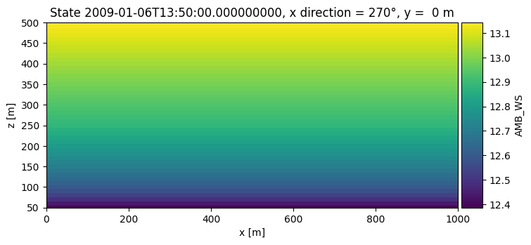
We now visualize the vertical flow profile for a single selected state:
with engine:
    farm_results = algo.calc_farm()
DefaultEngine: Selecting engine 'process'
ProcessEngine: Calculating 3000 states for 5 turbines
ProcessEngine: Starting calculation using 3 workers, for 3 states chunks.
ProcessEngine: Completed all 3 chunks
fr = farm_results.to_dataframe()
print(fr[[FV.WD, FV.REWS, FV.P]])
                                     WD      REWS            P
state               turbine
2009-01-01 00:00:00 0        340.144012  7.593225  1608.441679
                    1        340.144012  7.593225  1608.441679
                    2        340.144012  7.593225  1608.441679
                    3        340.144012  7.593225  1608.441679
                    4        340.144012  7.593225  1608.441679
...                                 ...       ...          ...
2009-01-21 19:50:00 0        201.682007  7.628299  1596.112474
                    1        201.682007  7.628299  1596.112474
                    2        201.682007  7.628299  1596.112474
                    3        201.682007  7.628299  1596.112474
                    4        201.682007  7.628299  1596.112474

[15000 rows x 3 columns]
with engine:
    o = foxes.output.FlowPlots2D(algo, farm_results)
    plot_data = o.get_states_data_xz(
        FV.AMB_WS,
        resolution=10,
        x_direction=270,
        xmin=0.0,
        xmax=1000.0,
        zmin=50.0,
        zmax=500.0,
        states_sel=["2009-01-06 13:50:00"],
    )

g = o.gen_states_fig_xz(plot_data, figsize=(8, 6))
fig = next(g)
plt.show()
States 'MultiHeightNCTimeseries': Reading file /home/runner/work/foxes/foxes/foxes/data/states/WRF-Timeseries-3000.nc
DefaultEngine: Selecting engine 'process'
ProcessEngine: Calculating data at 4646 points for 1 states
ProcessEngine: Starting calculation using 3 workers, for 1 states chunks and 3 targets chunks.
ProcessEngine: Completed all 3 chunks
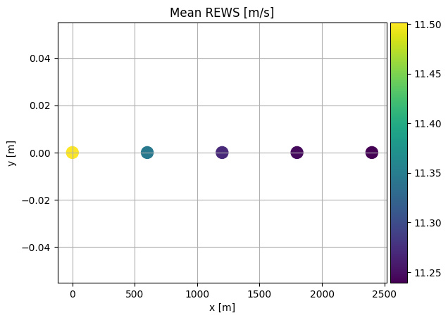
Let’s look at the mean REWS results for each turbine:
o = foxes.output.FarmLayoutOutput(farm, farm_results)
o.get_figure(color_by="mean_REWS", title="Mean REWS [m/s]", s=150, annotate=0)
plt.show()

o = foxes.output.FarmResultsEval(farm_results, algo=algo)
P0 = o.calc_mean_farm_power(ambient=True)
P = o.calc_mean_farm_power()
print(f"\nFarm power        : {P / 1000:.1f} MW")
print(f"Farm ambient power: {P0 / 1000:.1f} MW")
print(f"Farm efficiency   : {o.calc_farm_efficiency() * 100:.2f} %")
print(f"Annual farm yield : {o.calc_farm_yield():.2f} GWh")
Farm power        : 14.9 MW
Farm ambient power: 15.3 MW
Farm efficiency   : 97.35 %
Annual farm yield : 130.88 GWh