Single row of turbines
We start with the imports for this example:
%matplotlib inline
import numpy as np
import matplotlib.pyplot as plt

import foxes
import foxes.variables as FV
/home/runner/work/foxes/foxes/foxes/core/engine.py:4: TqdmExperimentalWarning: Using `tqdm.autonotebook.tqdm` in notebook mode. Use `tqdm.tqdm` instead to force console mode (e.g. in jupyter console)
  from tqdm.autonotebook import tqdm
The foxes setup is described in the Overview section. In summary, it consists of creating:
The so-called
model book, which contains all selectable modelsAmbient wind conditions, called
statesinfoxesterminologyThe
wind farm, collecting all turbine informationThe
algorithmwith its parameters and model choices
Here is a simple example for a single row of turbines along the x axis and a uniform wind speed with wind direction 270°:
# Create model book and add turbine type model:
# The csv file will be searched in the file system,
# and if not found, taken from static library.
#
# Note that we could actually skip adding the "NREL5"
# model and use "NREL5MW" which already exists in the
# default model book. Here this is for demonstrational
# purposes, in case you have your own turbine file:
mbook = foxes.ModelBook()
mbook.turbine_types["NREL5"] = foxes.models.turbine_types.PCtFile(
    "NREL-5MW-D126-H90.csv"
)

# create ambient wind conditions, a single uniform state:
states = foxes.input.states.SingleStateStates(ws=9.0, wd=270.0, ti=0.12, rho=1.225)

# create wind farm, a single row of turbines:
farm = foxes.WindFarm()
foxes.input.farm_layout.add_row(
    farm=farm,
    xy_base=[0.0, 0.0],
    xy_step=[800.0, 0.0],
    n_turbines=5,
    turbine_models=["NREL5"],
    verbosity=0,
)

# setup the calculation algorithm:
algo = foxes.algorithms.Downwind(
    farm,
    states,
    wake_models=["Jensen_linear_k007"],
    mbook=mbook,
    verbosity=0,
)
Now we can ask the algorithm object to run the calculation. This returns a xarray.Dataset object with results for each state and turbine:
farm_results = algo.calc_farm()
print("\nFarm results:\n", farm_results)
DefaultEngine: Selecting engine 'single'
SingleChunkEngine: Calculating 1 states for 5 turbines
SingleChunkEngine: Starting calculation using a single worker.
SingleChunkEngine: Completed all 1 chunks


Farm results:
 <xarray.Dataset> Size: 1kB
Dimensions:     (state: 1, turbine: 5)
Coordinates:
  * state       (state) int64 8B 0
Dimensions without coordinates: turbine
Data variables: (12/27)
    AMB_CT      (state, turbine) float64 40B 0.79 0.79 0.79 0.79 0.79
    AMB_P       (state, turbine) float64 40B 2.519e+03 2.519e+03 ... 2.519e+03
    AMB_REWS    (state, turbine) float64 40B 9.0 9.0 9.0 9.0 9.0
    AMB_REWS2   (state, turbine) float64 40B 9.0 9.0 9.0 9.0 9.0
    AMB_REWS3   (state, turbine) float64 40B 9.0 9.0 9.0 9.0 9.0
    AMB_RHO     (state, turbine) float64 40B 1.225 1.225 1.225 1.225 1.225
    ...          ...
    YAW         (state, turbine) float64 40B 270.0 270.0 270.0 270.0 270.0
    order       (state, turbine) int64 40B 0 1 2 3 4
    order_inv   (state, turbine) int64 40B 0 1 2 3 4
    order_ssel  (state, turbine) int64 40B 0 0 0 0 0
    weight      (state) float64 8B 1.0
    tname       (turbine) <U2 40B 'T0' 'T1' 'T2' 'T3' 'T4'
For a convenient summary printout we can easily convert the results into a pandas.DataFrame:
fr = farm_results.to_dataframe()
print(fr[[FV.WD, FV.AMB_REWS, FV.REWS, FV.TI, FV.AMB_P, FV.P, FV.CT]])
                  WD  AMB_REWS      REWS    TI   AMB_P            P        CT
state turbine
0     0        270.0       9.0  9.000000  0.12  2518.6  2518.600000  0.790000
      1        270.0       9.0  7.633459  0.12  2518.6  1557.076947  0.803665
      2        270.0       9.0  7.176627  0.12  2518.6  1290.332498  0.808234
      3        270.0       9.0  6.955794  0.12  2518.6  1167.325199  0.812210
      4        270.0       9.0  6.821354  0.12  2518.6  1106.880886  0.818932
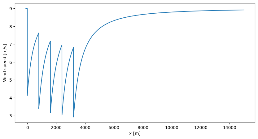
Once the farm calculation results are ready, we can evaluate the wake corrected flow and all points of interest. For example, we can evaluate the wind speed along the centre line:
# infer hub height from turbine type:
H = mbook.turbine_types["NREL5"].H

# create points of interest, shape (n_states, n_points, 3):
n_points = 8000
points = np.zeros((1, n_points, 3))
points[:, :, 0] = np.linspace(-100.0, 15000.0, n_points)[None, :]
points[:, :, 2] = H

# calculate point results:
point_results = algo.calc_points(farm_results, points)
print("\nPoint results:\n", point_results)

# create figure:
fig, ax = plt.subplots(figsize=(10, 5))
ax.plot(points[0, :, 0], point_results[FV.WS][0, :])
ax.set_xlabel("x [m]")
ax.set_ylabel("Wind speed [m/s]")
plt.show()
DefaultEngine: Selecting engine 'single'
SingleChunkEngine: Calculating data at 8000 points for 1 states
SingleChunkEngine: Starting calculation using a single worker.
SingleChunkEngine: Completed all 1 chunks


Point results:
 <xarray.Dataset> Size: 512kB
Dimensions:  (state: 1, point: 8000)
Coordinates:
  * state    (state) int64 8B 0
Dimensions without coordinates: point
Data variables:
    RHO      (state, point) float64 64kB 1.225 1.225 1.225 ... 1.225 1.225 1.225
    WD       (state, point) float64 64kB 270.0 270.0 270.0 ... 270.0 270.0 270.0
    TI       (state, point) float64 64kB 0.12 0.12 0.12 0.12 ... 0.12 0.12 0.12
    WS       (state, point) float64 64kB 9.0 9.0 9.0 9.0 ... 8.916 8.916 8.916
    AMB_RHO  (state, point) float64 64kB 1.225 1.225 1.225 ... 1.225 1.225 1.225
    AMB_WD   (state, point) float64 64kB 270.0 270.0 270.0 ... 270.0 270.0 270.0
    AMB_TI   (state, point) float64 64kB 0.12 0.12 0.12 0.12 ... 0.12 0.12 0.12
    AMB_WS   (state, point) float64 64kB 9.0 9.0 9.0 9.0 9.0 ... 9.0 9.0 9.0 9.0
    weight   (state) float64 8B 1.0
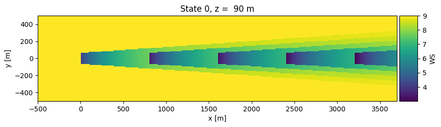
The foxes.output package provides a collection of standard outputs. For example, we can visualize the flow field in a horizontal slice at hub height:
o = foxes.output.FlowPlots2D(algo, farm_results)
plot_data = o.get_states_data_xy("WS", resolution=10, verbosity=0)
g = o.gen_states_fig_xy(plot_data, figsize=(10, 5))
fig = next(g)  # creates the figure for the next state, here there is only state 0
plt.show()
DefaultEngine: Selecting engine 'process'
ProcessEngine: Calculating data at 42521 points for 1 states
ProcessEngine: Starting calculation using 3 workers, for 1 states chunks and 3 targets chunks.
ProcessEngine: Completed all 3 chunks