Turbine-based ambient flow data
In some cases the inflow data is directly known at the turbine locations, in terms of (state, turbine)-type data. Such data can be simulated with foxes by using the TurbinePointCloud states class, as demonstrated here.
We start by importing the necessary packages and setting up the engine:
%matplotlib inline
import numpy as np
from xarray import Dataset, date_range
import matplotlib.pyplot as plt

import foxes
import foxes.variables as FV
/home/runner/work/foxes/foxes/foxes/core/engine.py:4: TqdmExperimentalWarning: Using `tqdm.autonotebook.tqdm` in notebook mode. Use `tqdm.tqdm` instead to force console mode (e.g. in jupyter console)
  from tqdm.autonotebook import tqdm
engine = foxes.Engine.new("default", verbosity=0)
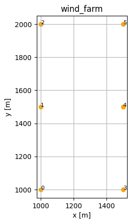
The first step is the creation of a regular grid of wind turbines:
n_turbines_x = 2
n_turbines_y = 3
n_turbines = n_turbines_x * n_turbines_y

farm = foxes.WindFarm()
foxes.input.farm_layout.add_grid(
    farm,
    xy_base=[1000, 1000],
    step_vectors=[[500, 0], [0, 500]],
    steps=[n_turbines_x, n_turbines_y],
    turbine_models=["DTU10MW"],
    verbosity=0,
)
o = foxes.output.FarmLayoutOutput(farm)
o.get_figure()
plt.show()
Next, let’s create an artificial Dataset object that represents data with (time, turbine) dimensions, representing a timeseries in January 2026 measured at he turbines of the above wind farm:
n_times = 10
times = date_range("2026-01-01", periods=n_times, freq="10min", unit="s")
times
DatetimeIndex(['2026-01-01 00:00:00', '2026-01-01 00:10:00',
               '2026-01-01 00:20:00', '2026-01-01 00:30:00',
               '2026-01-01 00:40:00', '2026-01-01 00:50:00',
               '2026-01-01 01:00:00', '2026-01-01 01:10:00',
               '2026-01-01 01:20:00', '2026-01-01 01:30:00'],
              dtype='datetime64[s]', freq='10min')
np.random.seed(42)

# Turbine i has wind speed (10 + i.x) m/s, where x grows linear with time
ws = np.zeros((n_times, n_turbines))
ws[:] = 10 + np.arange(n_turbines)[None, :]
ws += np.linspace(0, 1, n_times, endpoint=False)[:, None]

# the wind directions are randomly selected from a southern sector:
wd = np.random.uniform(0, 190, (n_times, n_turbines))

sdata = Dataset(
    coords={"time": times},
    data_vars={
        "ws": (("time", "turbine"), ws),
        "wd": (("time", "turbine"), wd),
        "ti": ("time", 0.1 + np.arange(n_times) / 100),
        "rho": ("turbine", 1.2 + np.arange(n_turbines) / 100),
    },
)
sdata
<xarray.Dataset> Size: 1kB
Dimensions:  (time: 10, turbine: 6)
Coordinates:
  * time     (time) datetime64[s] 80B 2026-01-01 ... 2026-01-01T01:30:00
Dimensions without coordinates: turbine
Data variables:
    ws       (time, turbine) float64 480B 10.0 11.0 12.0 13.0 ... 13.9 14.9 15.9
    wd       (time, turbine) float64 480B 71.16 180.6 139.1 ... 8.593 61.81
    ti       (time) float64 80B 0.1 0.11 0.12 0.13 0.14 0.15 0.16 0.17 0.18 0.19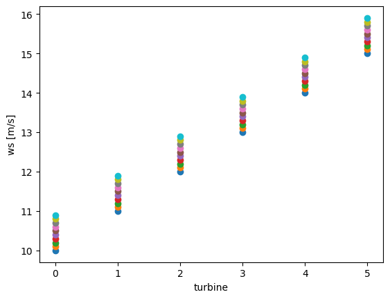
rho (turbine) float64 48B 1.2 1.21 1.22 1.23 1.24 1.25This is what the wind speed per turbine looks like, increasing linearly with time as described above:
for t in range(0, n_times):
    plt.scatter(sdata["turbine"], sdata["ws"][t])
plt.xticks(sdata["turbine"])
plt.xlabel("turbine")
plt.ylabel("ws [m/s]")
plt.show()
The data frame sdata is the base for our ambient states object:
states = foxes.input.states.TurbinePointCloud(
    data_source=sdata,
    states_coord="time",
    turbine_coord="turbine",
    output_vars=[FV.WS, FV.WD, FV.TI, FV.RHO],
    var2ncvar={
        FV.WS: "ws",
        FV.WD: "wd",
        FV.TI: "ti",
        FV.RHO: "rho",
    },
)
Next, let’s create the algorithm object:
algo = foxes.algorithms.Downwind(
    farm=farm,
    states=states,
    wake_models=["TurbOPark"],
    rotor_model="centre",
)
We now run the farm calculation:
with engine:
    farm_results = algo.calc_farm()
Initializing model 'TurbinePointCloud'

Initializing algorithm 'Downwind'

------------------------------------------------------------
  Algorithm: Downwind
  Running Downwind: calc_farm
------------------------------------------------------------
  n_states : 10
  n_turbines: 6
------------------------------------------------------------
  states    : TurbinePointCloud()
  rotor     : CentreRotor()
  controller: BasicFarmController()
  deflection: NoDeflection()
  wake frame: RotorWD()
  wake lngth: None
------------------------------------------------------------
  wakes:
    0) TurbOPark: TurbOParkWake(ws_quadratic, induction=Madsen, k=0.04*AMB_TI)
------------------------------------------------------------
  partial wakes:
    0) TurbOPark: axiwake6, PartialAxiwake(n=6)
------------------------------------------------------------
  turbine models:
    0) DTU10MW: PCtFile(D=178.3, H=119.0, P_nominal=10000.0, P_unit=kW, rho=1.225, var_ws_ct=REWS2, var_ws_P=REWS3)
------------------------------------------------------------


--------------------------------------------------
  Model oder
--------------------------------------------------
00) basic_ctrl
01) InitFarmData
02) centre
03) basic_ctrl
  03.0) Post-rotor: DTU10MW
04) SetAmbFarmResults
05) FarmWakesCalculation
06) ReorderFarmOutput
--------------------------------------------------


Input data:

 <xarray.Dataset> Size: 1kB
Dimensions:                  (state: 10, turbine: 6,
                              TurbinePointCloud_vars0: 2,
                              TurbinePointCloud_vars1: 1, tmodels: 1)
Coordinates:
  * state                    (state) datetime64[s] 80B 2026-01-01 ... 2026-01...
  * TurbinePointCloud_vars0  (TurbinePointCloud_vars0) <U2 16B 'WS' 'WD'
  * TurbinePointCloud_vars1  (TurbinePointCloud_vars1) <U2 8B 'TI'
  * tmodels                  (tmodels) <U7 28B 'DTU10MW'
Dimensions without coordinates: turbine
Data variables:
    TurbinePointCloud_data0  (state, turbine, TurbinePointCloud_vars0) float64 960B ...
    TurbinePointCloud_data1  (state, TurbinePointCloud_vars1) float64 80B 0.1...
    tmodel_sels              (state, turbine, tmodels) bool 60B True ... True


Farm variables: AMB_CT, AMB_P, AMB_REWS, AMB_REWS2, AMB_REWS3, AMB_RHO, AMB_TI, AMB_WD, AMB_YAW, CT, D, H, P, REWS, REWS2, REWS3, RHO, TI, WD, X, Y, YAW, order, order_inv, order_ssel, weight

Output variables: AMB_CT, AMB_P, AMB_REWS, AMB_REWS2, AMB_REWS3, AMB_RHO, AMB_TI, AMB_WD, AMB_YAW, CT, D, H, P, REWS, REWS2, REWS3, RHO, TI, WD, X, Y, YAW, order, order_inv, order_ssel, weight
DefaultEngine: Selecting engine 'single'
SingleChunkEngine: Calculating 10 states for 6 turbines
SingleChunkEngine: Starting calculation using a single worker.
SingleChunkEngine: Completed all 1 chunks
The results demonstrate that all data was correctly passed from the flow states to ambient variables:
farm_results.to_dataframe()[
    [FV.AMB_WD, FV.AMB_RHO, FV.AMB_TI, FV.AMB_REWS, FV.REWS, FV.P]
]
| AMB_WD | AMB_RHO | AMB_TI | AMB_REWS | REWS | P | ||
|---|---|---|---|---|---|---|---|
| state | turbine | ||||||
| 2026-01-01 00:00:00 | 0 | 71.162623 | 1.20 | 0.10 | 10.0 | 8.870120 | 5010.384802 |
| 1 | 180.635718 | 1.21 | 0.10 | 11.0 | 10.952161 | 9474.664608 | |
| 2 | 139.078849 | 1.22 | 0.10 | 12.0 | 8.375921 | 4307.026775 | |
| 3 | 113.745112 | 1.23 | 0.10 | 13.0 | 13.000000 | 10648.337500 | |
| 4 | 29.643542 | 1.24 | 0.10 | 14.0 | 14.000000 | 10641.826857 | |
| 5 | 29.638959 | 1.25 | 0.10 | 15.0 | 15.000000 | 10679.473520 | |
| 2026-01-01 00:10:00 | 0 | 11.035886 | 1.20 | 0.11 | 10.1 | 10.099999 | 7360.829038 |
| 1 | 164.573468 | 1.21 | 0.11 | 11.1 | 8.843683 | 5007.340784 | |
| 2 | 114.211852 | 1.22 | 0.11 | 12.1 | 11.307228 | 9972.847398 | |
| 3 | 134.533790 | 1.23 | 0.11 | 13.1 | 13.100000 | 10647.416250 | |
| 4 | 3.911054 | 1.24 | 0.11 | 14.1 | 14.100000 | 10646.284885 | |
| 5 | 184.282872 | 1.25 | 0.11 | 15.1 | 15.100000 | 10675.275344 | |
| 2026-01-01 00:20:00 | 0 | 158.164102 | 1.20 | 0.12 | 10.2 | 10.016835 | 7184.258808 |
| 1 | 40.344431 | 1.21 | 0.12 | 11.2 | 11.197560 | 9840.989324 | |
| 2 | 34.546744 | 1.22 | 0.12 | 12.2 | 11.338420 | 10002.152371 | |
| 3 | 34.846857 | 1.23 | 0.12 | 13.2 | 13.200000 | 10646.495000 | |
| 4 | 57.806026 | 1.24 | 0.12 | 14.2 | 14.200000 | 10650.742955 | |
| 5 | 99.703722 | 1.25 | 0.12 | 15.2 | 15.200000 | 10671.077167 | |
| 2026-01-01 00:30:00 | 0 | 82.069554 | 1.20 | 0.13 | 10.3 | 9.897905 | 6951.016997 |
| 1 | 55.333537 | 1.21 | 0.13 | 11.3 | 11.299817 | 9936.798585 | |
| 2 | 116.252050 | 1.22 | 0.13 | 12.3 | 12.228169 | 10641.088185 | |
| 3 | 26.503834 | 1.23 | 0.13 | 13.3 | 13.300000 | 10645.573750 | |
| 4 | 55.507483 | 1.24 | 0.13 | 14.3 | 14.300000 | 10655.201004 | |
| 5 | 69.608750 | 1.25 | 0.13 | 15.3 | 15.300000 | 10666.878991 | |
| 2026-01-01 00:40:00 | 0 | 86.653297 | 1.20 | 0.14 | 10.4 | 8.815365 | 4924.405208 |
| 1 | 149.183433 | 1.21 | 0.14 | 11.4 | 11.344388 | 9978.559102 | |
| 2 | 37.938019 | 1.22 | 0.14 | 12.4 | 12.398959 | 10642.691429 | |
| 3 | 97.704543 | 1.23 | 0.14 | 13.4 | 13.230629 | 10646.212826 | |
| 4 | 112.558768 | 1.24 | 0.14 | 14.4 | 13.468027 | 10643.690460 | |
| 5 | 8.825578 | 1.25 | 0.14 | 15.4 | 15.400000 | 10662.680814 | |
| 2026-01-01 00:50:00 | 0 | 115.433522 | 1.20 | 0.15 | 10.5 | 10.500000 | 8318.943186 |
| 1 | 32.399584 | 1.21 | 0.15 | 11.5 | 11.500000 | 10124.358512 | |
| 2 | 12.359803 | 1.22 | 0.15 | 12.5 | 12.500000 | 10643.639918 | |
| 3 | 180.288252 | 1.23 | 0.15 | 13.5 | 13.500000 | 10643.731250 | |
| 4 | 183.470086 | 1.24 | 0.15 | 14.5 | 12.322961 | 10642.606719 | |
| 5 | 153.595496 | 1.25 | 0.15 | 15.5 | 12.173622 | 10641.505264 | |
| 2026-01-01 01:00:00 | 0 | 57.876616 | 1.20 | 0.16 | 10.6 | 8.886403 | 5035.953749 |
| 1 | 18.557702 | 1.21 | 0.16 | 11.6 | 11.600000 | 10218.052941 | |
| 2 | 130.004275 | 1.22 | 0.16 | 12.6 | 11.252646 | 9921.565977 | |
| 3 | 83.628974 | 1.23 | 0.16 | 13.6 | 13.568073 | 10643.104132 | |
| 4 | 23.187265 | 1.24 | 0.16 | 14.6 | 14.600000 | 10668.575151 | |
| 5 | 94.083613 | 1.25 | 0.16 | 15.6 | 15.600000 | 10654.284461 | |
| 2026-01-01 01:10:00 | 0 | 6.533819 | 1.20 | 0.17 | 10.7 | 10.607070 | 8575.405397 |
| 1 | 172.770876 | 1.21 | 0.17 | 11.7 | 11.026436 | 9653.068240 | |
| 2 | 49.168197 | 1.22 | 0.17 | 12.7 | 11.814770 | 10449.692396 | |
| 3 | 125.879234 | 1.23 | 0.17 | 13.7 | 13.700000 | 10641.888750 | |
| 4 | 59.225104 | 1.24 | 0.17 | 14.7 | 14.700000 | 10673.033200 | |
| 5 | 98.812924 | 1.25 | 0.17 | 15.7 | 15.700000 | 10650.086285 | |
| 2026-01-01 01:20:00 | 0 | 103.874953 | 1.20 | 0.18 | 10.8 | 10.800000 | 9037.527277 |
| 1 | 35.122347 | 1.21 | 0.18 | 11.8 | 11.548786 | 10170.068407 | |
| 2 | 184.221079 | 1.22 | 0.18 | 12.8 | 12.251232 | 10641.304685 | |
| 3 | 147.275236 | 1.23 | 0.18 | 13.8 | 13.800000 | 10640.967500 | |
| 4 | 178.504799 | 1.24 | 0.18 | 14.8 | 14.799416 | 10677.465227 | |
| 5 | 170.017197 | 1.25 | 0.18 | 15.8 | 14.137962 | 10649.667015 | |
| 2026-01-01 01:30:00 | 0 | 113.600996 | 1.20 | 0.19 | 10.9 | 10.899155 | 9275.030750 |
| 1 | 175.156105 | 1.21 | 0.19 | 11.9 | 11.529127 | 10151.648575 | |
| 2 | 16.813575 | 1.22 | 0.19 | 12.9 | 12.897184 | 10647.368358 | |
| 3 | 37.236744 | 1.23 | 0.19 | 13.9 | 12.873414 | 10647.474504 | |
| 4 | 8.593185 | 1.24 | 0.19 | 14.9 | 14.900000 | 10681.949298 | |
| 5 | 61.812763 | 1.25 | 0.19 | 15.9 | 15.900000 | 10641.985129 |
For completeness, the states results at off-turbine evaluation points will be interpolated by point cloud methods.