Power mask
This example demonstrates how to derate or boost turbines by using a turbine model called PowerMask. We need the following imports:
%matplotlib inline
import numpy as np
import pandas as pd
import matplotlib.pyplot as plt

import foxes
import foxes.variables as FV
import foxes.constants as FC
/home/runner/work/foxes/foxes/foxes/core/engine.py:6: TqdmExperimentalWarning: Using `tqdm.autonotebook.tqdm` in notebook mode. Use `tqdm.tqdm` instead to force console mode (e.g. in jupyter console)
  from tqdm.autonotebook import tqdm
We start by creating a simple states table, this time via a pandas.DataFrame object:
sdata = pd.DataFrame(index=range(8))
sdata.index.name = FC.STATE
sdata[FV.WS] = [5.0, 8.0, 11.0, 14.0, 18.0, 20.0, 22.0, 25.0]
print(sdata)

states = foxes.input.states.StatesTable(
    data_source=sdata,
    output_vars=[FV.WS, FV.WD, FV.TI, FV.RHO],
    fixed_vars={FV.WD: 270.0, FV.TI: 0.05, FV.RHO: 1.225},
)
         WS
state
0       5.0
1       8.0
2      11.0
3      14.0
4      18.0
5      20.0
6      22.0
7      25.0
Next, we create the power mask for these states. The idea is that for each state and turbine, we can set a maximal power value in a table.
If the calculated power value is above this value, the turbine is derated.
If the maximal power exceeds the nominal power of the turbine type and the calculated value is at nominal power, then the turbine is boosted to the maximal power value.
If the maximal power value in the power mask is
NaN, then the turbine is neither derated nor boosted (normal operation)
Again we create a DataFrame that contains the power mask data:
pmask = pd.DataFrame(index=sdata.index, columns=[f"PMax_{i}" for i in range(5)])
pmask.loc[np.s_[:4], "PMax_4"] = 1000
pmask.loc[np.s_[4:], "PMax_4"] = 6000
pmask.loc[np.s_[2:], "PMax_2"] = 3000
pmask.loc[0, "PMax_0"] = 300.0
pmask.loc[3, "PMax_0"] = 1000.0
print(pmask)
       PMax_0 PMax_1 PMax_2 PMax_3 PMax_4
state
0       300.0    NaN    NaN    NaN   1000
1         NaN    NaN    NaN    NaN   1000
2         NaN    NaN   3000    NaN   1000
3      1000.0    NaN   3000    NaN   1000
4         NaN    NaN   3000    NaN   6000
5         NaN    NaN   3000    NaN   6000
6         NaN    NaN   3000    NaN   6000
7         NaN    NaN   3000    NaN   6000
Using this data we can now create the model book. Notice how the variable FV.MAX_P is set to the above values via the turbine model SetFarmVars:
mbook = foxes.models.ModelBook()
mbook.turbine_models["set_Pmax"] = foxes.models.turbine_models.SetFarmVars()
mbook.turbine_models["set_Pmax"].add_var(FV.MAX_P, pmask)
We can now create a wind farm that consists of 5 turbines in a row. Some thoughts about the turbine_models argument:
The actual
PowerMaskturbine model is pre-defined in the defaultModelBookunder the namePMask, so we can just add it to the turbine model list.It should appear after the turbine type model
NREL5, sincePMaskcorrects the results od the latter.Furthermore,
PMaskshould be placed somewhere after the above created turbine modelset_Pmaxin the list of turbine models, such that the values of the variableFV.MAX_Pare present at the time whenPMaskis called.The models
NREL5andset_Pmaxhave no influence on each other, so their order does not matter.
We choose the following pattern:
models = ["NREL5MW", "set_Pmax", "PMask"]

farm = foxes.WindFarm()
foxes.input.farm_layout.add_row(
    farm,
    xy_base=[0.0, 0.0],
    xy_step=[600.0, 0.0],
    n_turbines=5,
    turbine_models=models,
)
Turbine 0, T0: xy=(0.00, 0.00), NREL5MW, set_Pmax, PMask
Turbine 1, T1: xy=(600.00, 0.00), NREL5MW, set_Pmax, PMask
Turbine 2, T2: xy=(1200.00, 0.00), NREL5MW, set_Pmax, PMask
Turbine 3, T3: xy=(1800.00, 0.00), NREL5MW, set_Pmax, PMask
Turbine 4, T4: xy=(2400.00, 0.00), NREL5MW, set_Pmax, PMask
We can now setup our algorithm and run the calculation:
algo = foxes.algorithms.Downwind(
    farm,
    states,
    rotor_model="centre",
    wake_models=["Bastankhah2014_linear_k002"],
    mbook=mbook,
    verbosity=0,
)
# run calculation with power mask:
farm_results = algo.calc_farm()

fr = farm_results.to_dataframe()
print(fr[[FV.WD, FV.AMB_REWS, FV.REWS, FV.MAX_P, FV.AMB_P, FV.P]])

o = foxes.output.FarmResultsEval(farm_results, algo=algo)
P0 = o.calc_mean_farm_power(ambient=True)
P = o.calc_mean_farm_power()
print(f"\nFarm power: {P / 1000:.1f} MW, Efficiency = {P / P0 * 100:.2f} %")

# this output is needed later:
o1 = foxes.output.StateTurbineMap(farm_results)
DefaultEngine: Selecting engine 'single'
SingleChunkEngine: Calculating 8 states for 5 turbines
SingleChunkEngine: Starting calculation using a single worker.
SingleChunkEngine: Completed all 1 chunks

                  WD  AMB_REWS       REWS    MAXP   AMB_P            P
state turbine
0     0        270.0       5.0   5.000000   300.0   300.0   300.000000
      1        270.0       5.0   3.814381     NaN   403.9   152.233017
      2        270.0       5.0   3.004124     NaN   403.9    41.065774
      3        270.0       5.0   2.701086     NaN   403.9     0.000000
      4        270.0       5.0   3.393368  1000.0   403.9    94.470023
1     0        270.0       8.0   8.000000     NaN  1771.1  1771.100000
      1        270.0       8.0   5.128471     NaN  1771.1   446.770655
      2        270.0       8.0   4.359237     NaN  1771.1   258.959385
      3        270.0       8.0   4.099815     NaN  1771.1   200.278202
      4        270.0       8.0   3.951750  1000.0  1000.0   171.080144
2     0        270.0      11.0  11.000000     NaN  4562.5  4562.500000
      1        270.0      11.0   7.077374     NaN  4562.5  1232.378551
      2        270.0      11.0   6.019489  3000.0  3000.0   746.362135
      3        270.0      11.0   5.535864     NaN  4562.5   582.717698
      4        270.0      11.0   5.273676  1000.0  1000.0   495.225773
3     0        270.0      14.0  14.000000  1000.0  1000.0  1000.000000
      1        270.0      14.0  13.700036     NaN  5000.0  5000.000000
      2        270.0      14.0  11.839741  3000.0  3000.0  3000.000000
      3        270.0      14.0  10.930815     NaN  5000.0  4485.421327
      4        270.0      14.0   7.961950  1000.0  1000.0  1000.000000
4     0        270.0      18.0  18.000000     NaN  5000.0  5000.000000
      1        270.0      18.0  17.187504     NaN  5000.0  5000.000000
      2        270.0      18.0  16.463311  3000.0  3000.0  3000.000000
      3        270.0      18.0  16.261366     NaN  5000.0  5000.000000
      4        270.0      18.0  15.581278  6000.0  6000.0  6000.000000
5     0        270.0      20.0  20.000000     NaN  5000.0  5000.000000
      1        270.0      20.0  19.377548     NaN  5000.0  5000.000000
      2        270.0      20.0  18.860383  3000.0  3000.0  3000.000000
      3        270.0      20.0  18.740478     NaN  5000.0  5000.000000
      4        270.0      20.0  18.324505  6000.0  6000.0  6000.000000
6     0        270.0      22.0  22.000000     NaN  5000.0  5000.000000
      1        270.0      22.0  21.479296     NaN  5000.0  5000.000000
      2        270.0      22.0  21.069694  3000.0  3000.0  3000.000000
      3        270.0      22.0  20.983152     NaN  5000.0  5000.000000
      4        270.0      22.0  20.671550  6000.0  6000.0  6000.000000
7     0        270.0      25.0  25.000000     NaN  5000.0  5000.000000
      1        270.0      25.0  24.716577     NaN  5000.0  5000.000000
      2        270.0      25.0  24.480543  3000.0  3000.0  3000.000000
      3        270.0      25.0  24.420013     NaN  5000.0  5000.000000
      4        270.0      25.0  24.230301  6000.0  6000.0  6000.000000

Farm power: 15.2 MW, Efficiency = 87.64 %
For a visualization of the results, let’s re-run the case without the power mask:
# reset, for run calculation without power mask:
for t in farm.turbines:
    t.models.remove("set_Pmax")
    t.models.remove("PMask")
farm_results = algo.calc_farm()
o0 = foxes.output.StateTurbineMap(farm_results)
DefaultEngine: Selecting engine 'single'
SingleChunkEngine: Calculating 8 states for 5 turbines
SingleChunkEngine: Starting calculation using a single worker.
SingleChunkEngine: Completed all 1 chunks
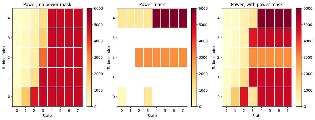
We are now in the position to create plots that compare the turbine power results, using the two output objects o0 and o1:
# show power:
fig, axs = plt.subplots(1, 3, figsize=(15, 5))
o0.plot_map(
    FV.P,
    ax=axs[0],
    edgecolor="white",
    title="Power, no power mask",
    cmap="YlOrRd",
    vmin=0,
    vmax=np.nanmax(pmask),
)
o1.plot_map(
    FV.MAX_P,
    ax=axs[1],
    edgecolor="white",
    cmap="YlOrRd",
    title="Power mask",
    vmin=0,
    vmax=np.nanmax(pmask),
)
o1.plot_map(
    FV.P,
    ax=axs[2],
    edgecolor="white",
    cmap="YlOrRd",
    title="Power, with power mask",
    vmin=0,
    vmax=np.nanmax(pmask),
)
plt.show()
Similarly, for the thrust coefficients:
# show ct:
fig, axs = plt.subplots(1, 3, figsize=(15, 5))
o0.plot_map(
    FV.CT,
    ax=axs[0],
    edgecolor="white",
    title="ct, no power mask",
    cmap="YlGn",
    vmin=0,
    vmax=1.0,
)
o1.plot_map(
    FV.MAX_P,
    ax=axs[1],
    edgecolor="white",
    cmap="YlOrRd",
    title="Power mask",
    vmin=0,
    vmax=np.nanmax(pmask),
)
o1.plot_map(
    FV.CT,
    ax=axs[2],
    edgecolor="white",
    cmap="YlGn",
    title="ct, with power mask",
    vmin=0,
    vmax=1.0,
)
plt.show()
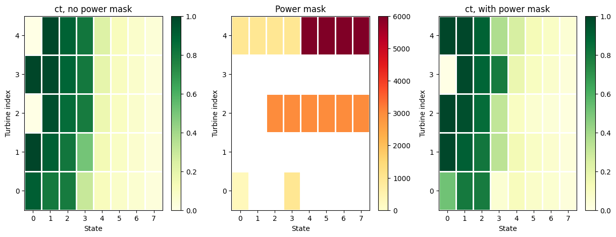
The above visualizations demonstrate that the power mask has effects on both the produced power and ct. Hence, also wakes are affected by derating and boosts.
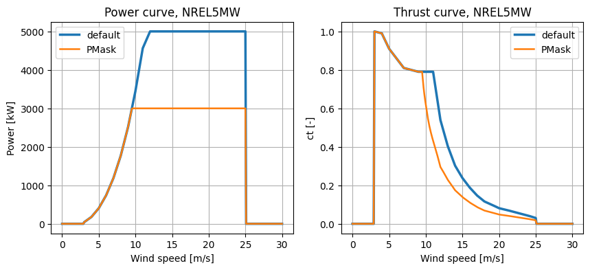
We can also visualize the effect of the PowerMask model on power and thrust curve, here for the case of derating from 5 MW to 3 MW:
o = foxes.output.TurbineTypeCurves(mbook)
plot_data = o.calc_plot_data("NREL5MW", [FV.P, FV.CT], P_max=3000.0)
fig, axs = plt.subplots(1, 2, figsize=(10, 4))
o.plot_curves(plot_data, axs=axs)
plt.show()
DefaultEngine: Selecting engine 'single'
SingleChunkEngine: Calculating 301 states for 1 turbines
SingleChunkEngine: Starting calculation using a single worker.
SingleChunkEngine: Completed all 1 chunks

DefaultEngine: Selecting engine 'single'
SingleChunkEngine: Calculating 301 states for 1 turbines
SingleChunkEngine: Starting calculation using a single worker.
SingleChunkEngine: Completed all 1 chunks