Timeseries data
In this example we calculate the data of a wind farm with 67 turbines in a time series containing 8000 uniform inflow states.
The required imports are:
%matplotlib inline
import matplotlib.pyplot as plt

import foxes
import foxes.variables as FV
/home/runner/work/foxes/foxes/foxes/core/engine.py:4: TqdmExperimentalWarning: Using `tqdm.autonotebook.tqdm` in notebook mode. Use `tqdm.tqdm` instead to force console mode (e.g. in jupyter console)
  from tqdm.autonotebook import tqdm
First, we create the states. The data_source can be any csv-type file (or pandas readable equivalent), or a pandas.DataFrame object. If it is a file path, then it will first be searched in the file system, and if not found, in the static data. If it is also not found there, an error showing the available static data file names is displayed.
In this example the static data file timeseries_8000.csv.gz will be used, with content
Time,ws,wd,ti
2017-01-01 00:00:00,15.62,244.06,0.0504
2017-01-01 00:30:00,15.99,243.03,0.0514
2017-01-01 01:00:00,16.31,243.01,0.0522
2017-01-01 01:30:00,16.33,241.26,0.0523
...
Notice the column names, and how they appear in the Timeseries constructor:
states = foxes.input.states.Timeseries(
    data_source="timeseries_8000.csv.gz",
    output_vars=[FV.WS, FV.WD, FV.TI, FV.RHO],
    var2col={FV.WS: "ws", FV.WD: "wd", FV.TI: "ti"},
    fixed_vars={FV.RHO: 1.225},
)
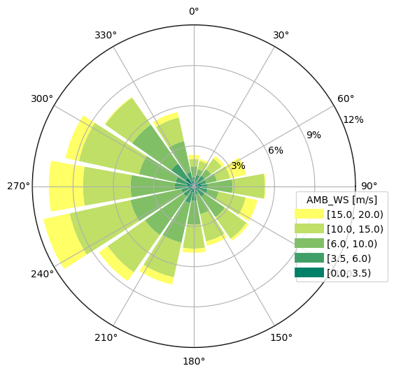
We can visualize the wind distribution via the StatesRosePlotOutput. Here we display the ambient wind speed in a wind rose with 16 wind direction sectors and 5 wind speed bins:
o = foxes.output.StatesRosePlotOutput(states, point=[0.0, 0.0, 100.0])
o.get_figure(16, FV.AMB_WS, [0, 3.5, 6, 10, 15, 20], figsize=(6, 6))
plt.show()
DefaultEngine: Selecting engine 'single'
SingleChunkEngine: Calculating 8000 states for 1 turbines
SingleChunkEngine: Starting calculation using a single worker.
SingleChunkEngine: Completed all 1 chunks
For the time series with uniform data, any choice of the point argument will produce the same figure.
Next, we create the example wind farm with 67 turbines from static data. The file test_farm_67.csv has the following structure:
index,label,x,y
0,T0,101872.70,1004753.57
1,T1,103659.97,1002993.29
2,T2,100780.09,1000779.97
3,T3,100290.42,1004330.88
...
For more options, check the API section foxes.input.farm_layout.
We consider two turbine models in this example: the wind turbine type NREL5MW and the turbine model kTI_02, both from the default model book. The latter model adds the variable k for each state and turbine, calculated as k = kTI * TI, with constant kTI = 0.2. The parameter k will later be used by the wake model.
farm = foxes.WindFarm()
foxes.input.farm_layout.add_from_file(
    farm, "test_farm_67.csv", turbine_models=["NREL5MW"], verbosity=0
)
Next, we create the algorithm, with further model selections. In particular, two wake models are invoked, the model Bastankhah_quadratic for wind speed deficits and the model CrespoHernandez_max for turbulence intensity:
algo = foxes.algorithms.Downwind(
    farm,
    states,
    rotor_model="centre",
    wake_models=["Bastankhah2014_quadratic_ka02", "CrespoHernandez_max_ka04"],
    verbosity=0,
)
Also notice the chunks parameter, specifying that always 1000 states should be considered in vectorized form during calculations. The progress is automatically visualized when invoking the DaskRunner:
farm_results = algo.calc_farm()

fr = farm_results.to_dataframe()
print("\n", fr[[FV.WD, FV.AMB_REWS, FV.REWS, FV.AMB_P, FV.P]])
DefaultEngine: Selecting engine 'process'
ProcessEngine: Calculating 8000 states for 67 turbines
ProcessEngine: Starting calculation using 3 workers, for 3 states chunks.
ProcessEngine: Completed all 3 chunks
                                  WD  AMB_REWS       REWS    AMB_P            P
state               turbine
2017-01-01 00:00:00 0        244.06     15.62  15.610500  5000.00  5000.000000
                    1        244.06     15.62  14.012903  5000.00  5000.000000
                    2        244.06     15.62  15.021033  5000.00  5000.000000
                    3        244.06     15.62  15.560020  5000.00  5000.000000
                    4        244.06     15.62  14.564008  5000.00  5000.000000
...                             ...       ...        ...      ...          ...
2017-06-16 15:30:00 62       299.19     11.70   8.145984  4868.75  1880.222715
                    63       299.19     11.70  11.490711  4868.75  4777.186188
                    64       299.19     11.70  11.700000  4868.75  4868.750000
                    65       299.19     11.70  11.642754  4868.75  4843.705093
                    66       299.19     11.70   8.055085  4868.75  1812.276034

[536000 rows x 5 columns]
Let’s evaluate the results:
# add capacity factor and efficiency to farm_results:
o = foxes.output.FarmResultsEval(farm_results, algo=algo)
o.add_capacity_factor()
o.add_capacity_factor(ambient=True)
o.add_efficiency()

# print results by turbine:
turbine_results = o.reduce_states()
turbine_results[FV.AMB_YLD] = o.calc_yield(annual=True, ambient=True)
turbine_results[FV.YLD] = o.calc_yield(annual=True)
turbine_results[FV.EFF] = turbine_results[FV.P] / turbine_results[FV.AMB_P]
print("\nResults by turbine:\n")
print(turbine_results)

# print power results:
P0 = o.calc_mean_farm_power(ambient=True)
P = o.calc_mean_farm_power()
print(f"\nFarm power        : {P / 1000:.1f} MW")
print(f"Farm ambient power: {P0 / 1000:.1f} MW")
print(f"Farm efficiency   : {o.calc_farm_efficiency():.2f}")
print(f"Annual farm yield : {turbine_results[FV.YLD].sum():.2f} GWh")
Capacity factor added to farm results
Ambient capacity factor added to farm results
Efficiency added to farm results

Results by turbine:

           AMB_CT         AMB_P   AMB_REWS  AMB_REWS2  AMB_REWS3  AMB_RHO  \
turbine
0        0.593832  2.454179e+07  10.142951  10.142951  10.142951    1.225
1        0.593832  2.454179e+07  10.142951  10.142951  10.142951    1.225
2        0.593832  2.454179e+07  10.142951  10.142951  10.142951    1.225
3        0.593832  2.454179e+07  10.142951  10.142951  10.142951    1.225
4        0.593832  2.454179e+07  10.142951  10.142951  10.142951    1.225
...           ...           ...        ...        ...        ...      ...
62       0.593832  2.454179e+07  10.142951  10.142951  10.142951    1.225
63       0.593832  2.454179e+07  10.142951  10.142951  10.142951    1.225
64       0.593832  2.454179e+07  10.142951  10.142951  10.142951    1.225
65       0.593832  2.454179e+07  10.142951  10.142951  10.142951    1.225
66       0.593832  2.454179e+07  10.142951  10.142951  10.142951    1.225

           AMB_TI      AMB_WD     AMB_YAW        CT  ...         YAW  \
turbine                                              ...
0        0.056837  214.291794  214.291794  0.629342  ...  214.291794
1        0.056837  214.291794  214.291794  0.648618  ...  214.291794
2        0.056837  214.291794  214.291794  0.622579  ...  214.291794
3        0.056837  214.291794  214.291794  0.622090  ...  214.291794
4        0.056837  214.291794  214.291794  0.640959  ...  214.291794
...           ...         ...         ...       ...  ...         ...
62       0.056837  214.291794  214.291794  0.634036  ...  214.291794
63       0.056837  214.291794  214.291794  0.637352  ...  214.291794
64       0.056837  214.291794  214.291794  0.614525  ...  214.291794
65       0.056837  214.291794  214.291794  0.641752  ...  214.291794
66       0.056837  214.291794  214.291794  0.642317  ...  214.291794

             order  order_inv   order_ssel         CAPF     AMB_CAPF  \
turbine
0        30.747125  31.543750  1332.833375  4222.251300  4908.357436
1        29.423750  37.537250  1332.833375  3679.225291  4908.357436
2        33.122125  32.728875  1332.833375  4103.081737  4908.357436
3        34.077750  33.087375  1332.833375  4175.812673  4908.357436
4        31.093875  29.326000  1332.833375  3828.742434  4908.357436
...            ...        ...          ...          ...          ...
62       31.599000  37.140000  1332.833375  3932.475484  4908.357436
63       35.948000  30.083750  1332.833375  3896.693678  4908.357436
64       39.153125  33.625125  1332.833375  4410.534587  4908.357436
65       27.239750  31.799375  1332.833375  3812.884197  4908.357436
66       28.507375  29.193875  1332.833375  3853.811458  4908.357436

              EFF  tname    AMB_YLD        YLD
turbine
0        0.860217     T0  26.873257  23.116826
1        0.749584     T1  26.873257  20.143758
2        0.835938     T2  26.873257  22.464373
3        0.850756     T3  26.873257  22.862574
4        0.780046     T4  26.873257  20.962365
...           ...    ...        ...        ...
62       0.801180    T62  26.873257  21.530303
63       0.793890    T63  26.873257  21.334398
64       0.898576    T64  26.873257  24.147677
65       0.776815    T65  26.873257  20.875541
66       0.785153    T66  26.873257  21.099618

[67 rows x 31 columns]

Farm power        : 166.3 MW
Farm ambient power: 205.5 MW
Farm efficiency   : 0.81
Annual farm yield : 1456.42 GWh
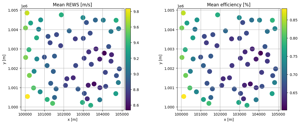
We can visualize the mean rotor equivalent wind speed as seen by each turbine and also the mean efficiency with respect to the time series data as colored layout plots:
fig, axs = plt.subplots(1, 2, figsize=(14, 5))
o = foxes.output.FarmLayoutOutput(farm, farm_results)
o.get_figure(
    fig=fig, ax=axs[0], color_by="mean_REWS", title="Mean REWS [m/s]", s=150, annotate=0
)
o.get_figure(
    fig=fig,
    ax=axs[1],
    color_by="mean_EFF",
    title="Mean efficiency [%]",
    s=150,
    annotate=0,
)
plt.show()